Chapter 3

3.1 (Informal) Set definition

The number of elements of a finite set $A$ is called it’s cardinality and is denoted $|A|$.

3.2 Set Equality

$A=B\stackrel{\text{def}}{⟺}\forall x(x\in A\leftrightarrow x\in B)$.

3.1 Single element sets

For any sets $a$ and $b$, $\{a\}=\{b\}⟹a=b$

Ordered Pairs

We can model ordered pairs (tuples) by defining $(a,b)\stackrel{\text{def}}{=}\{\{a\},\{a,b\}\}$

Set-Builder Notation

We can write a set in the following two ways:

• $\{x\in S|P(x)\}$ lists all $x\in S$ for which the predicate $P(x)$ is true
• $\{f(x)|x\in S\}$ lists the images of all $x$ by function $f$ for all $x\in S$.

Subsets

3.3 Subset

The set $A$ is a subset of the the set $B$ denoted $A\subseteq B$ if every element of $A$ is also an element of $B$, $A\subseteq B\stackrel{\text{def}}{⟺}\forall x(x\in A\to x\in B)$

3.2 Equality as double Subset

$A=B⟺(A\subseteq B)\wedge (B\subseteq A)$

3.3 Transitivity of Subsets

$(A\subseteq B)\wedge (B\subseteq C)⟹A\subseteq C$

3.4 Union and Intersection

The union of two sets $A$ and $B$ is defined as $A\cup B\stackrel{\text{def}}{=}\{x|x\in A\vee x\in B\}$ and their intersection is defined as $A\cap B\stackrel{\text{def}}{=}\{x|x\in A\wedge x\in B\}$

This can be extended to several sets, where $\bigcup \mathcal{A}\stackrel{\text{def}}{=}\{x|x\in A\text{for some}A\in \mathcal{A}\}$ and $\bigcap \mathcal{A}\stackrel{\text{def}}{=}\{x|x\in A\text{for all}A\in \mathcal{A}\}$

3.5 Difference of two Sets

The difference of two sets $A$ and $B$, denoted $B\setminus A$ is the set of elements that are in $B$ without being in $A$: $B\setminus A\stackrel{\text{def}}{=}\{x\in B|x\notin A\}$

3.4 Laws of union and intersection

Idempotence: $A\cap A=A$; $A\cup A=A$;

Commutativity: $A\cap B=B\cap A$; $A\cup B=B\cup A$;

Associativity: $A\cap (B\cap C)=(A\cap B)\cap C$; $A\cup (B\cup C)=(A\cup B)\cup C$;

Absorption: $A\cap (A\cup B)=A$; $A\cup (A\cap B)=A$;

Distributivity: $A\cap (B\cup C)=(A\cap B)\cup (A\cap C)$; $A\cup (B\cap C)=(A\cup B)\cap (A\cup C)$;

Consistency: $A\subseteq B⟺A\cap B=A⟺A\cup B=B$.

It is intuitive to think about operations on sets like logical operations:

• $\cup \sim \vee$ and $\cap \sim \wedge$
• $\subseteq \sim \to$ and the other way around.

Empty set

3.6 Empty Set

A set is called empty if it contains no elements $\forall x\neg (x\in A)$

3.5 Uniqueness of the Empty Set

There is only one empty set, which is often denoted $\varnothing$ or $\{\}$.

3.6 The empty set is a subset of every set

$\forall A(\varnothing \subseteq A)$

Constructing the Natural Numbers

We can construct the natural numbers using the following definitions from empty sets: $0\stackrel{\text{def}}{=}\varnothing$, $1\stackrel{\text{def}}{=}\{\varnothing \}$, $2\stackrel{\text{def}}{=}\{\varnothing ,\{\varnothing \}\}$, etc…

Natural number $\text{n}$

The successor of any number is then $s(\text{n})\stackrel{\text{def}}{=}\text{n}\cup \{\text{n}\}$.

Power Set

3.7 Power Set

The power set of a set $A$, denoted $\mathcal{P}(A)$ is the set of all subsets of $A$: $\mathcal{P}(A)\stackrel{\text{def}}{=}\{S|S\subseteq A\}$

Cardinality of the Power set

For a finite set with cardinality $k$, the power set has cardinality $2^k$ (hence the name power set and alternative notation $2^A$).

Cartesian Product of Sets

3.8 Cartesian Product

The Cartesian Product $A\times B$ of two sets $A$ and $B$ is the set of all ordered pairs with the first component from $A$ and the second component from $B$: $A\times B=\{(a,b)|a\in A\wedge b\in B\}$

Cardinality of Cartesian product

The cardinaliity of $|A\times B|=|A|\cdot |B|$

The Cartesian product is not associative and ${\text{bigtimes}}_{i=1}^3{A}_i\ne (A_1\times A_2)\times A_3$ The first would give $(a_1,a_2,a_3)$, the second $((a_1,a_2),a_3)$.

Relations

3.9 Binary Relation

A (binary) relation $\rho$ from a set $A$ to a set $B$ (also called an ($A$, $B$)-relation) is a subset of $A\times B$. If $A=B$, then $\rho$ is called a relation on $A$.

Instead of $(a,b)\in \rho$ one usually writes $a\rho b$ .

3.10 Identity relation

For any set $A$, the identity relation on $A$, denoted ${\text{id}}_A$ or simply id) is the relation ${\text{id}}_A=\{(a,a)|a\in A\}$.

Number of relations on a finite set

On a set of cardinality $|A|$ there are $2^{|\mathcal{P}(A)|}=2^{2^{|A|}}$ possible distinct relations. This is because $\rho \subseteq \mathcal{P}(A)$.

We can represent any relation $\rho$ from finite sets $A\times B$ as a boolean matrix $M^{\rho }\in {\mathbb{R}}^{|A|\times |B|}$. If $(a,b)\in \rho$ then the corresponding matrix entry if set to $1$.

We can also represent relations as a directed graph, the nodes of which correspond to the elements of $A$ and $B$ while the edges represent relations.

3.11 Inverse of a relation

The inverse of a relation $\rho \subseteq A\times B$ is the relation $\hat{\rho }\subseteq B\times A$ defined by $\hat{\rho }\stackrel{\text{def}}{=}\{(b,a)|(a,b)\in \rho \}$

In the matrix representation, the inverse corresponds to the transpose. In the graph representation, the inverse if reversing the direction of all edges.

The inverse of the inverse being equal to the element itself needs to be re-proven every time we want to use it (in the exam for example)!

Example On the set $\mathbb{Z}$, the inverse of the relation $\le$ is the relation $\ge$.

3.12 Composition of Relations

Let $\rho$ be a relation from $A$ to $B$ and let $\sigma$ be a relation from $B$ to $C$. Then the composition of $\rho$ and $\sigma$, denoted $\rho \circ \sigma$ (or also $\rho \sigma$) is the relation from $A$ to $C$ defined by: $\rho \circ \sigma \stackrel{\text{def}}{=}\{(a,c)|\exists b((a,b)\in \rho \wedge (b,c)\in \sigma )\}$

The $n$-fold composition of a relation $\rho$ on a set $A$ with itself is denoted ${\rho }^n$.

Example If $\varphi$ is the parenthood relation on the set $H$ of all humans, then ${\varphi }^2$ is the grand-parenthood relation.

In the matrix representation, composition is matrix multiplication. In the graph representation, the composition corresponds to the natural composition of two graphs, there is a path from $a$ to $c$ if there is a path from $a$ to $b$ in graph $1$ and $b$ to $c$ in graph $2$.

3.7 Associativity of composition

The composition of relations is associative, i.e., we have $\rho \circ (\sigma \circ \varphi )=(\rho \circ \sigma )\circ \varphi$.

3.8 Inverse of composition

Let $\rho$ be a relation from $A$ to $B$ and let $\sigma$ be a relation from $B$ to $C$. Then the inverse: $\widehat{\rho \sigma }=\hat{\sigma }\hat{\rho }$

Properties of relations

Reflexivity

3.13 Reflexivity

A relation $\rho$ on a set $A$ is called reflexive if $a\rho a$ is true for all $a\in A$, i.e. if $\text{id}\subseteq \rho$

3.14 Irreflexivity

A relation $\rho$ on a set $A$ is called irreflexive if $a/\rho a$ is true for all $a\in A$, i.e. if $\rho \cap \text{id}=\varnothing$

Example The relations $\le ,\ge ,|$ on $\mathbb{Z}$ are reflexive, but $<,>$ are not.

The relation is reflexive if it contains the identity matrix, otherwise irreflexive.

Symmetry

3.15 Symmetry

A relation $\rho$ on a set $A$ is called symmetric if $a\rho b⟺b\rho a$ is true for all $a,b\in A$, i.e. if $\rho =\hat{\rho }$

Example The relation ${\equiv }_m$ on $\mathbb{Z}$ is symmetric.

You can easily see that in matrix representation this corresponds to the transpose being equal to itself, i.e. the definition of a symmetric matrix.

3.16 Antisymmetry

A relation $\rho$ on a set $A$ is called antisymmetric if $a\rho b\wedge b\rho a⟺a=b$ is true for all $a,b\in A$, i.e. if $\rho \cap \hat{\rho }\subseteq \text{id}$

Example The relations $\le ,\ge$ are antisymmetric. Example The relation $|$ on $\mathbb{N}$ is antisymmetric as if $a|b\wedge b|a\Rightarrow a=b$ but on $\mathbb{Z}$ it is not as the negative of an element divides it’s positive counterpart.

This is equal to the matrix not being symmetric. In the graph representation this means that there is not a single cycle of length 2, no edge from $a$ to $b$ and $b$ to $a$.

Note that antisymmetric is not the negation of symmetry. A relation (for example the relation $=$) can be both at the same time.

Transitivity

3.17 Transitivity

A relation $\rho$ on a set $A$ is called transitive if $a\rho b\wedge b\rho c⟹a\rho c$ is true for all $a,b,c\in A$.

Example The relations $\le ,\ge ,<,>,|,{\equiv }_m$ are all transitive on $\mathbb{Z}$.

3.9 Transitivity of self-composition

A relation $\rho$ is transitive if and only if ${\rho }^2\subseteq \rho$. This is intuitive if $k$-ary self-composition is viewed as finding paths of length $k$ in the graph.

Transitive Closure

3.18 Transitive Closure

The transitive closure of a relation $\rho$ on a set $A$, denoted ${\rho }^{\ast }$ is ${\rho }^{\ast }={\bigcup }_{n\in \mathbb{N}\setminus \{0\}}{\rho }^n$

You can view the transitive closure as the “reachability relation” which is only true for a pair $a,b$ if there is a path of finite length from $a$ to $b$ in relation $\rho$.

Equivalence Relations

3.19 Equivalence Relation

An equivalence relation is a relation on a set $A$ that is reflexive, symmetric and transitive.

3.20 Equivalence Classes

For an equivalence relation $\theta$ on a set $A$ and for $a\in A$, the set of elements of $A$ that are equivalent to $a$ is called the equivalence class of $a$ and is denoted as $[a{]}_{\theta }$: $[a{]}_{\theta }\stackrel{\text{def}}{=}\{b\in A|b\theta a\}$

Example The equivalence classes of ${\equiv }_3$ are the sets $[0]=\{\dots ,-6,-3,0,3,6,\dots \}$, $[1]=\{\dots ,-5,-2,1,4,7,\dots \}$ and $[2]=\{\dots ,-4,-1,2,5,8,\dots \}$.

There are two trivial equivalence classes: the complete relation $A\times A$, for which there is a single equivalence class $A$ and the identity relation for which the equivalence classes are all singletons $\{a\}$.

3.10 Intersection of two Equivalence relations (on the same $A$)

The intersection of two equivalence relations (on the same set) is an equivalence relation.

Example The intersection of ${\equiv }_5\cap {\equiv }_3={\equiv }_{15}$.

Partitions

3.21 Partition of a set

A partition of a set $A$ is a set of mutually disjoint subsets of $A$ that cover $A$, i.e. a set $\{S_i|i\in \mathcal{I}\}$ (for some index set $\mathcal{I}$) satisfying $S_i\cap S_j=\varnothing \text{for}i\ne j\text{and}{\bigcup }_{i\in \mathcal{I}}{S}_i=A$

Partitions and equivalence classes capture the same relationship.

3.22 Quotient Set

The set of equivalence classes of an equivalence relation $\theta$, denoted by $A/\theta \stackrel{\text{def}}{=}\{[a{]}_{\theta }|a\in A\}$ is called the quotient set of $A$ by $\theta$ or simply $A$ modulo $\theta$, or $A$ mod $\theta$.

3.11 Equivalence classes form a partition

The set $A/\theta$ of equivalence classes of an equivalence relation $\theta$ on $A$ is a partition of $A$.

Definition of the rational numbers

Consider the set $A=\mathbb{Z}\times (\mathbb{Z}\setminus \{0\})$ and the equivalence relation $\sim$ defined as follows $(a,b)\sim (c,d)\stackrel{\text{def}}{⟺}ad=bc$ This relation is reflexive, symmetric and transitive. All pairs $(u,v)\in [(a,b)]$ correspond to the same rational number and all equivalence classes correspond to distinct equivalence classes.

$\mathbb{Q}\stackrel{\text{def}}{=}(\mathbb{Z}\times (\mathbb{Z}\setminus \{0\}))/\sim$

Partial Order Relations

The definition of a partial order is the same as that for an equivalence class, we simply replace the symmetry condition by an antisymmetry condition.

Partial order

A partial order (or simply an order relation) on a set $A$ is a relation that is reflexive, antisymmetric and transitive. A set $A$ together with a partial order $⪯$ on $A$ is called a partially ordered set (or simply poset) and is denoted as $(A;⪯)$.

Example An example for a poset would be $(\mathbb{Z};\le )$ or $\ge$. $<$ is not a partial order as it’s not reflexive. Example The subset relation on the power set of $A$ is a partial order: $(\mathcal{P}(A);\subseteq )$ is a poset. Example The relation $=$ is both an equivalence relation and a partial order relation.

In the graph representation, a partial order has no cycles (transitive, but no symmetry).

Equal and strict

For any relation $⪯$, $\prec$ is defined as $a⪯b\wedge a\ne b$.

3.24 Comparable and Incomparable

For a poset $(A;⪯)$, two elements $a$ and $b$ are comparable if $a⪯b$ or $b⪯a$; otherwise they are called incomparable.

3.25 Totally and partially ordered

If any two elements of a poset $(A;⪯)$ are comparable, then $A$ is called totally ordered (all elements can be compared) (or linearly ordered) by $⪯$.

Example $(\mathbb{Z};\le )$ is a totally ordered poset. So is any subset of $\mathbb{Z}$ for the relation $\le ,\ge$. Example The poset $(\mathcal{P}(A);\subseteq )$ is not totally ordered if $|A|\ge 2$ (see $\{2,3\}⊈\{3,4\}$ nor $\{3,4\}⊈\{2,3\}$). Example The poset $(\mathbb{N};|)$ is not totally ordered ($2\nmid 3\wedge 3\nmid 2$).

Hasse Diagrams

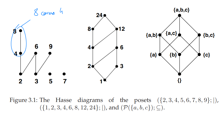
3.26 Covering

In a poset $(A;⪯)$ an element $b$ is said to cover an element $a$ if $a\prec b$ and there exists not $c$ with $a\prec c$ and $c\prec b$ (i.e. between $a$ and $b$).

Example In a hierarchy $b$ covering $a$ means that $b$ is the direct superior of $a$.

3.27 Hasse Diagram

The Hasse Diagram of a (finite) poset $(A;⪯)$ is the directed graph whose vertices are labeled with the elements of $A$ and where there is an edge from $a$ to $b$ if and only if $b$ covers $a$.

Posets and Lexicographic Order

3.28 Direct Product

The direct product of posets $(A;⪯)$ and $(B;⊑)$, denoted $(A;⪯)\times (B;⊑)$, is the set $A\times B$ with the relation $\le$ (on $A\times B$) defined by $(a_1,b_1)\le (a_2,b_2)\stackrel{\text{def}}{⟺}{a}_1⪯a_2\wedge b_1⊑b_2$

3.12 Direct Product of Posets is a Poset

$(A;⪯)\times (B;⊑)$ is a poset.

Lexicographic order

For given posets $(A;⪯)$ and $(B;⊑)$, the relation ${\le }_{\text{lex}}$ defined on $A\times B$ by $(a_1,b_1){\le }_{\text{lex}}(a_2,b_2)\stackrel{\text{def}}{⟺}{a}_1⪯a_2\vee (a_1=a_2\wedge b_1⊑b_2)$ is a partial order relation.

This is useful as if both the first and second posets are totally ordered, then so is the lexicographic order on $A\times B$.

Example This is how a phone book or a dictionary would be ordered.

Special Elements in Posets

Special Elements of Posets

Definition 3.29. Let $(A;⪯)$ be a poset, and let $S\subseteq A$ be some subset of $A$. Then

1. $a\in A$ is a minimal (maximal) element of $A$ if there exists no $b\in A$ with $b\prec a$ $(b\succ a)$.
2. $a\in A$ is the least (greatest) element of $A$ if $a⪯b$ $(a⪰b)$ for all $b\in A$.
3. $a\in A$ is a lower (upper) bound of $S$ if $a⪯b$ $(a⪰b)$ for all $b\in S$.
4. $a$ is the greatest lower bound (least upper bound) of $S$ if $a$ is the greatest (least) element of the set of all lower (upper) bounds of $S$

The greatest lower bound and least upper bound are sometimes denoted $\text{glb}(S)$ and $\text{lub}(S)$.

Example The poset $(\{2,3,4,5,6,7,8,9\};|)$ has no least or greatest elements (as not all are comparable). $2,3,5,7$ are minimal elements. $5,6,7,8,9$ are maximal elements. The number $2$ is the lower bound (even the greatest lower bound) of the subset $\{4,6,8\}$. $\{4,9\}$ has no lower (nor upper) bound.

3.30 Well-Ordering

A poset $(A;⪯)$ is well-ordered if it is totally ordered and if every non-empty subset of A has a least element.

Every totally ordered finite poset is well-ordered. The property of well ordering is of interest only for infinite posets. $\mathbb{N}$ is well ordered by $\le$. Any subset of a well-ordered set is well-ordered (by the same relation).

Meet, Join and Lattices

3.31 Meet and Join

Let $(A;⪯)$ be a poset. If $a$ and $b$ (i.e. the set of $\{a,b\}\subseteq A$) have a greatest lower bound, then it is called the meet of $a$ and $b$, often denoted $a\wedge b$. If $a$ and $b$ have a least upper bound, then it is called the join of $a$ and $b$, often denoted $a\vee b$.

3.32 Lattices

A poset $(A;⪯)$ in which every pair of elements has a meet and join is called a lattice.

Example The posets $(\mathbb{N};\le )$, $|$ and $(\mathcal{P}(S);\subseteq )$ are lattices. Example The poset $(\{1,2,3,4,5,6,8,12,24\};|)$ is a lattice. The meet of two elements is their gcd, while their join is the lcm. $6\wedge 8=2,6\vee 8=24,3\wedge 4=1,3\vee 4=12$.

Functions

Functions are a special type of relation.

3.33 Functions

A function $f:A⟶B$ from a domain $A$ to a codomain $B$ is a relation from $A$ to $B$ with the special properties (using the relation notation $afb$):

1. $\forall a\in A\exists b\in Bafb$ ($f$ is totally defined)
2. $\forall a\in A\forall b,b^{\prime }\in B(afb\wedge af{b}^{\prime }\to b=b^{\prime })$ ($f$ is well defined)

3.34 Set of all functions

The set of all functions $A\to B$ is denoted as $B^A$.

3.35 Partial functions

A partial function $A\to B$ is a relation from $A$ to $B$ such that only condition 2. of def 3.33 holds ($\forall a\in A\forall b,b^{\prime }\in B(afb\wedge af{b}^{\prime }\to b=b^{\prime })$, $f$ is well defined).

Two partial functions are equal if they are equal as relations (they agree for all arguments).

3.36 Image

For a function $f:A\to B$ and a subset $S$ of $A$, the image of $S$ under $f$, denoted $f(S)$, is the set $f(S)\stackrel{\text{def}}{=}\{f(a)|a\in S\}$

3.37 Image or Range

The subset $f(A)$ of $B$ is called the image (or range) or $f$ and is also denoted $Im(f)$.

Example The function $f:\mathbb{R}\to \mathbb{R}$ defined by $f(x)=x^2$ has as it’s range the set ${\mathbb{R}}^{\ge 0}$.

3.38 Preimage

For a subset $T$ of $B$, the preimage of $T$, denoted $f^{-1}(T)$ is the set of values in $A$ that map into $T$: $f^{-1}(T)\stackrel{\text{def}}{=}\{a\in A|f(a)\in T\}$

Example The preimage of the interval $[4,9]$ is $[-3,-2]\cup [2,3]$.

3.39 Injectivity, Surjectivity and Bijectivity

A function $f:A\to B$ is called 1 ) injective (or one-to-one or an injection) if for $a\ne a^{\prime }$ we have $f(a)\ne f(a^{\prime })$, i.e. no two distinct values are mapped to the same function value (there are no “collisions”). 2) surjective (or onto) if $f(A)=B$, i.e. for every $b\in B,b=f(a)$ for some $a\in A$ (every value in the codomain is taken on for some argument). 3) bijective (or a bijection) if it is both injective and surjective.

Proving Injectivity and Surjectivity:

• Injectivity:
  • Assume that $a\ne b$ and show that if $f(a)=f(b)⟹a=b$ which is a contradiction
• Surjectivity:
  • $\forall b\in B$ show that we can find an a such that $f(a)=b$
  • $f(x)=2x:\mathbb{Z}\to \mathbb{Z}$, let $b=7\in \mathbb{Z}$, but there is no $a=b/2\in \mathbb{Z}$ thus not surjective.

3.40 Inverse of a bijection

For a bijective function $f$, the inverse (as a relation) is called the inverse function of $f$, usually noted as $f^{-1}$.

3.41 Composition

The composition of a function $f:A\to B$ and a function $g:B\to C$ denoted by $g\circ f$ or simply $gf$ is defined by $(g\circ f)(a)=g(f(a))$

Composition of functions and properties

1. The composition of two injective functions is an injective function
2. The composition of two surjective functions is a surjective function
3. The composition of two bijective functions is a bijective function

Function Composition Order

4. Order of application: In $g\circ f$, function $f$ is applied FIRST, then $g$

• Read right to left: $g\circ f$ means “first do $f$, then do $g$”

• $(g\circ f)(a)$ = apply $f$ to $a$ first, getting $f(a)$, then apply $g$ to result

2. Different from relation composition:

• Relations: $\rho \circ \sigma$ where $\rho :A\to B$ and $\sigma :B\to C$ (same order)
• Functions: $g\circ f$ where $f:A\to B$ and $g:B\to C$ (reversed notation)

Memory Aid: In $g\circ f$, the order of letters (left to right) is OPPOSITE to order of application (right to left).

3.14 Associativity of function composition

Function composition is associative, i.e. $(h\circ g)\circ f=h\circ (g\circ f)$.

Countable and Uncountable Sets

3.42 Equinumerous, dominates, countable and uncountable

(i) Two sets $A$ and $B$ are equinumerous, denoted $A\sim B$, if there exists a bijection $A\to B$. (ii) The set $B$ dominates the set $A$, denoted $A⪯B$ if $A\sim C$ for some subset $C\subseteq B$ or, equivalently, if there exists an injection $A\to B$. (iii) A set $A$ is countable if $A\subseteq \mathbb{N}$ and uncountable otherwise.

Example The set $\mathbb{Z}$ is countable and $\mathbb{Z}\sim \mathbb{N}$ by the bijection $f(n)=(-1{)}^n\lceil n/2\rceil$.

Strict Smaller Cardinality

We say that $A$ has a strictly smaller cardinality than $B$ if $A\prec B\wedge A\nsim B$. There’s an injection but no bijection from $A$ to $B$.

3.15 Relations and Countability

(i) The relation $\sim$ is an equivalence relation. (ii) The relation $⪯$ is transitive: $A⪯B\wedge B⪯C\iff A⪯C$. (iii) $A\subseteq B\Rightarrow A⪯B$.

Countable

$A$ is countable if $A\sim \mathbb{N}$ or $A\sim \text{n}$ for an $n\in \mathbb{N}$, i.e. $\text{n}=\{0,1,2,3,\dots ,n-1\}$.

3.16 Definition of $\sim$

$A⪯B\wedge B⪯A\Rightarrow A\sim B$ is the Cantor-Bernstein-Schroeder Theorem.

Between finite and countably infinite

For any finite sets $A$ and $B$, we have $A\sim B$ if and only if $|A|=|B|$. A finite set never has the cardinality as one of it’s proper subsets.

This is not true for infinite sets however, as $\text{O}$ the set of odd numbers $\text{O}\sim \mathbb{N}$ as there exists a bijection between both sets, $f(n)=2n+1$.

3.17 Countable Sets

A set $A$ is countable if and only if it is finite or if $A\sim \mathbb{N}$.

This means that there is no cardinality level between finite and countably infinite.

Well-Ordering Principle of $\mathbb{N}$.

Every set of natural numbers has a least element. This fact is called the well-ordering principle of $\mathbb{N}$.

Important Countable Sets

3.18 Finite binary sequences

The set $\{0,1{\}}^{\ast }\stackrel{\text{def}}{=}\{ϵ,0,1,00,01,10,11,000,\dots \}$ of finite binary sequences is countable.

3.19 Product of ${\mathbb{N}}^2$ is countable

The set $\mathbb{N}\times \mathbb{N}(={\mathbb{N}}^2)$ of ordered pairs of natural numbers is countable.

3.20 Cartesian product of any countable sets is countable

The Cartesian product $A\times B$ of two countable sets $A$ and $B$ is countable, i.e. $A⪯\mathbb{N}\wedge B⪯\mathbb{N}\Rightarrow A\times B⪯\mathbb{N}$.

3.21 $\mathbb{Q}$ is countable

The rational numbers $\mathbb{Q}$ are countable.

3.22 Countable sets

Let $A$ and $A_i$ for $i\in \mathbb{N}$ be countable sets. (i) For any $n\in \mathbb{N}$, the set $A^n$ of $n$-tuples over $A$ is countable. (ii) The union ${\bigcup }_{i\in \mathbb{N}}{A}_i$ of a countable list $A_0,A_1,A_2,\dots$ of countable sets is countable. (iii) The set $A^{\ast }$ of finite sequences of elements from $A$ is countable.

Uncountability of $\{0,1{\}}^{\infty }$.

3.43 Definition of $\{0,1{\}}^{\infty }$

Let $\{0,1{\}}^{\infty }$ denote the set of semi-infinite binary sequences or, equivalently, the set of functions $\mathbb{N}\to \{0,1\}$.

*Note that the difference between $\{0,1{\}}^{\infty }$ and $\{0,1{\}}^{\ast }$ is that all elements in the first have infinite length, while the second considers elements of all lengths.

3.23 Uncountability of $\{0,1{\}}^{\infty }$

The set $\{0,1{\}}^{\infty }$ is uncountable.

This can be proven by Cantor’s diagonalisation argument. We can write $\{0,1{\}}^{\mathbb{N}}$ instead of $\{0,1{\}}^{\infty }$.

We also can show that $[0,1]$ is uncountable und thus $\mathbb{R}$ is too.

To prove the uncountability of a set $A$, we use the following proof schema: 2. By Injection - Show an injection from $B\to A$ ($B⪯A$) and that $B$ is uncountable, ex: $B=\{0,1{\}}^{\infty }$. - You can use any known uncountable sets: $\{0,1{\}}^{\infty },\mathbb{R},[0,1],\mathcal{P}(\mathbb{N})$ - If $A$ was countable ($\iff A⪯\mathbb{N}$), then by the transitivity of $⪯$ this would imply that $B⪯\mathbb{N}$ which is a contradiction as $B$ is known uncountable. 3. By Diagonalisation - Assume uncountability and show a contradiction (ex: Diagonalisation)

4-Schritt Muster für Uncountability:

• Injektion finden: Konstruiere $f:\{0,1{\}}^{\infty }\to A$, sodass $b\ne b^{\prime }⟹f(b)\ne f(b^{\prime })$
• Funktion verifizieren: Zeige dass $f$ well-defined und total ist, und $f(b)\in A$ für alle $b$.
• Injektivität beweisen: Zeige $f(b)=f(b^{\prime })⟹b=b^{\prime }$ oder direkt $b\ne b^{\prime }⟹f(b)\ne f(b^{\prime })$.
• Schluss: $\{0,1{\}}^{\infty }⪯A$. Annahme $A⪯\mathbb{N}$ führt zu Widerspruch via Transitivität.

Tricks:

• Complement Trick: Zeige $A\subseteq B$ ($B$ uncountable), $B\backslash A$ countable $⟹A$ uncountable. (You have to prove this in the exam.)
  • Assume $A$ is countable towards contradiction.
  • Show that $B\backslash A$ is countable as well under this assumption.
  • Thus $A\cup (B\backslash A)$ also countable (Theorem 3.22: Union of countable is countable).
  • But $A\cup (B\backslash A)=B$ which is uncountable - contradiction!
• Verwende $\mathbb{R}$ oder $[0,1]$ statt $\{0,1{\}}^{\infty }$ falls einfacher.

Uncomputable functions

3.44 Computable functions

A function $f:\mathbb{N}\to \{0,1\}$ is called computable if there is a program that, for every $n\in \mathbb{N}$, when given $n$ as input, outputs $f(n)$.

3.24 Uncomputable functions

There are uncomputable functions $\mathbb{N}\to \{0,1\}$.

This can be proven by thinking about computer programs as bitstrings. As the set of finite bitstrings $\{0,1{\}}^{\ast }$ is countable, while the set of functions $\mathbb{N}\to \{0,1\}$ is not, there must be uncomputable functions.

The Halting problem is a prominent example of an uncomputable function. It is undecidable.

Bemerkung der Lecture am 27.10.2025

Wir haben $\mathbb{N}\prec \mathcal{P}(\mathbb{N})\prec \mathcal{P}(\mathcal{P}(\mathbb{N}))$. In fact the power set of any set dominates that set.

We also have the Kontinuumshypothese which states that there is no $M$ such that $\mathbb{N}\prec M\prec \{0,1{\}}^{\infty }$.