Chapter 4

This chapter deals with some basics regarding number theory. It in particular focuses on the natural/whole numbers, but the concepts can be applied to any Field.

Prerequisites

We assume that the concepts of $\mathbb{Z}$, addition, multiplication, negation, associativity, commutativity, distributivity, $\le$ and $|\dots |$ are clear.

4.2 Divisors and Division

4.1 Divides

We say that $a$ divides $b$ for any integers (denoted $a|b$) if $\exists c\in \mathbb{Z}b=ac$. $a$ is a divisor (de: Teiler) of $b$, $b$ a multiple (de: Vielfaches) of $a$ and $c$ the quotient (de: Quotient).

Every non-zero integer is a divisor of $0$. Moreover $1$ and $-1$ are divisors of every integer.

We define a prime as $p\text{prime}\stackrel{\text{def}}{\iff }p>1\wedge \forall d((d>1)\wedge (d|p)\to d=p)$.

4.1 Euclidean Division

For all integers $a$ and $d\ne 0$ there exist unique integers $q$ and $r$ satisfying $a=dq+r\text{and}0\le r\le |d|$

$r$ is called the remainder (de: Rest).

4.2 Greatest Common Divisor

For integers $a$ and $b$ (not both $0$), an integer $d$ is called a greatest common divisor of $a$ and $b$ if $d$ divides both $a$ and $b$ and if every common divisor of $a$ and $b$ divides $d$, i.e. if $d|a\wedge d|b\wedge \forall c((c|a\wedge c|b)\to c|d)$

4.3 GCD

For $a,b\in \mathbb{Z}$ (not both 0), one denotes the unique postive greatest common divisor by $\text{gcd}(a,b)$ and usually calls it the greatest common divisor. If $\text{gcd}(a,b)=1$, then $a$ and $b$ are called relatively prime.

Proof $pq|a$ if $p$ and $q$ are coprime.

This is an important result for the exam: $p\mid a\wedge q\mid a\wedge \gcd (p,q)=1⟹pq\mid a$ Which is the same as saying $\exists k\in \mathbb{Z}$ such that $a=pq\cdot k$. Since $p\mid a$ and $q\mid a$, we have: $\exists k,k^{\prime }\in \mathbb{Z}\text{ such that }a=pk\wedge a=q{k}^{\prime }$ Since $\gcd (p,q)=1$, by Bézout’s identity: $\exists u,v\in \mathbb{Z}\text{ such that }1=pu+qv$ Now we can write: \begin{align} a &= 1 \cdot a \\ &= a \cdot (pu + qv) \\ &= pua + qva \\ &= pu \cdot qk' + qv \cdot pk \\ &= pq(uk' + vk') \end{align} Thus $pq\mid a$. $\square$

4.2 GCD relations

For any integers $m,n$ and $q$ we have $\text{gcd}(m,n-qm)=\text{gcd}(m,n)$

This implies the necessary step for Euclid’s algorithm $\text{gcd}(m,R_m(n))=\text{gcd}(m,n)$

4.4 Ideals

For $a,b\in \mathbb{Z}$, the ideal generated by $a$ and $b$, denoted $(a,b)$, is the set $(a,b)\stackrel{\text{def}}{=}\{ua+vb|u,v\in \mathbb{Z}\}$ Similarly, for a single integer we have $(a)\stackrel{\text{def}}{=}\{ua|u\in \mathbb{Z}\}$

4.3 All ideals can be generated by a single integer

For $a,b\in \mathbb{Z}$ there exists $d\in \mathbb{Z}$ such that $(a,b)=(d)$. This implies that every ideal can be generated by a single integer.

4.4 GCD

Let $a,b\in \mathbb{Z}$ (not both 0). If $(a,b)=(d)$, then $d$ is a greatest common divisor of $a$ and $b$.

4.5 GCD result of ideal

For $a,b\in \mathbb{Z}$ (not both $0$), the exist $u,v\in \mathbb{Z}$ such that $\text{gcd}(a,b)=ua+vb$

This is Bézout’s identity.

There is an algorithm (Euclidean algorithm) which can be used to find the values of $u$ and $v$ for this decomposition. It works by computing the euclidean decomposition $a=bq+r$ and replacing $a$ by $r$ in $gcd(a,b)$, rince and repeat until you arrive at $gcd(m,0)$. Then you can use back propagation to find the values for the equation $1=\dots$. Knowing this algorithm is necessary for the exam!

Walk-through: $\gcd (252,198)=18$

1. Gleichungen der Reste:
   • $54=252-1\cdot 198$
   • $36=198-3\cdot 54$
   • $18=54-1\cdot 36$
2. Rückwärtssubstitution:
   • $18=54-1\cdot 36$
   • $18=54-1\cdot (198-3\cdot 54)=4\cdot 54-1\cdot 198$
   • $18=4\cdot (252-1\cdot 198)-198=4\cdot 252-5\cdot 198$ Ergebnis: $x=4$ und $y=-5$

4.5 Least common multiple

The least common multiple $l$ of two positive integers $a$ and $b$, denoted $l=\text{lcm}(a,b)$, is the common multiple of $a$ and $b$ which divides every common multiple of $a$ and $b$, i.e. $a|l\wedge b|l\wedge \forall m((a|m\wedge b|m)\to l|m)$

4.3 Primes

4.6 Primes

A positive integer $p>1$ is called prime if the only positive divisors of $p$ are $1$ and $p$ itself. An integer greater than $1$ that is not prime is called composite.

4.6 Fundamental theorem of arithmetic

Every positive integer can be written uniquely (up to the order in which factors are listed) as the product of primes. $x=\prod p_i^{e_i}$

We need to state this theorem when decomposing any integer into it’s prime factors!

4.7 Prime divides one in product

If $p$ is a prime which divides he product $x_1{x}_2\dots x_n$ of some integers $x_1,\dots ,x_n$, then $p$ divides one of them, i.e. $p|x_i$ for some $i\in \{1,\dots ,n\}$

We can now express the $\text{gcd}$ and $\text{lcm}$ in this form. Let $a$ and $b$ be

$a={\prod }_i{p}_i^{e_i}\text{and}b={\prod }_i{p}_i^{f_i}$

Then $\text{gcd}(a,b)={\prod }_i{p}_i^{\text{min}(e_i,f_i)}$ and

$\text{lcm}(a,b)={\prod }_i{p}_i^{\text{max}(e_i,f_i)}$ We can also see that $\text{gcd}(a,b)\cdot \text{lcm}(a,b)=ab$ as $\text{min}(e_i,f_i)+\text{max}(e_i,f_i)=e_i+f_i$.

4.9 Infinity of primes

There are infinitely many primes.

4.10 Prime density

Gaps between primes can be arbitrarily large, i.e. for every $k\in \mathbb{N}$, there exists $n\in \mathbb{N}$ such that the set $\{n,n+1,\dots ,n+k-1\}$ contains no prime.

4.7 Prime counting function

The prime counting function $\pi :\mathbb{R}\to \mathbb{N}$ is defined as follows: For any real $x,\pi (x)$ is the number of primes $\le x$.

4.11 Prime counting function limit

${\lim }_{x\to \infty }\frac{\pi (x)\ln (x)}{x}=1$

To test whether a number is prime, we have to test every smaller integer which could be a divisor, there is one shortcut however.

4.12 Prime divisors

Every composite integer $n$ has a prime divisor $\le \sqrt{n}$.

Congruences and Modulo Arithmetic

4.8 Congruence

For $a,b,m\in \mathbb{Z}$ with $m\ge 1$ , we say that $a$ is congruent to $b$ modulo $m$ if $m$ divides $a-b$. We write $a\equiv b(\text{mod}m)$ or simply $a{\equiv }_{m}b$, i.e., $a{\equiv }_{m}b\stackrel{\text{def}}{\iff }m|(a-b)$

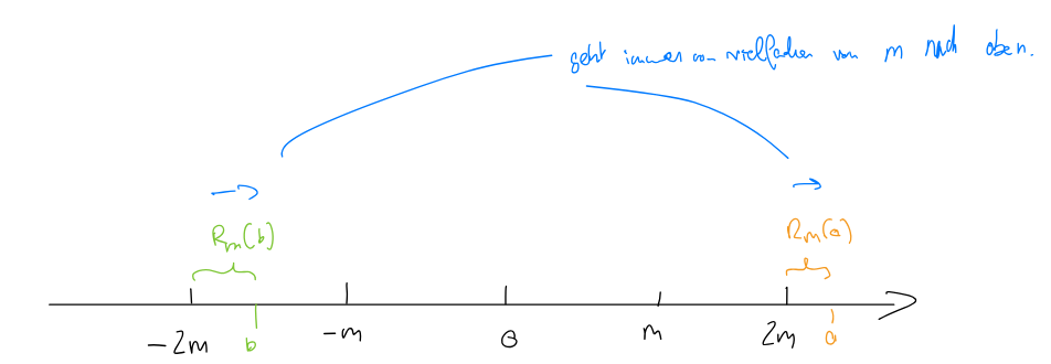
We define the function $R_m(x)$ as the smallest positive $n\in \mathbb{N}$ for which $x{\equiv }_{m}n$.

4.13 Modulo Equivalence Relation

For any $m>1$, ${\equiv }_m$ is an equivalence relation on $\mathbb{Z}$.

4.14 Modular arithmetic

If $a{\equiv }_{m}b$ and $c{\equiv }_{m}d$ then $a+c{\equiv }_{m}b+d\text{and}ac{\equiv }_{m}bd$

Simplifying calculations

4.15 Modular reduction of a multivariate polynomial

Let $f(x_1,\dots ,x_k)$ be a multi-variate polynomial in $k$ variables with integer coefficients, and let $m\ge 1$. If $a_i{\equiv }_m{b}_i$ for $1\le i\le k$, then $f(a_1,\dots ,a_k){\equiv }_{m}f(b_1,\dots ,b_k)$

We are often interested in only the remainder of an integer calculation. We want the result to be bounded below the $m$ we are moduloing against. We can use the fact that ${\equiv }_m$ is an equivalence relation and since there are $m$ equivalence classes ${\equiv }_m$ namely $[0],[1],\dots ,[m-1]$. Each class has a smallest, natural representative $R_m(a)\in [a]$ in the set ${\mathbb{Z}}_m:=\{0,\dots ,m-1\}$.

4.16 $R_m$

For any $a,b,m\in \mathbb{Z}$ with $m\ge 1$, $\text{(i)}a{\equiv }_m{R}_m(a)$ $\text{(ii)}a{\equiv }_{m}b⟺R_m(a)=R_m(b)$

Together these two properties imply that:

4.17 Polynomial reduction

Let $f(x_1,\dots ,x_k)$ be a multi-variate polynomial in $k$ variables with integer coefficients, and let $m\ge 1$. Then $R_m(f(a_1,\dots ,a_k))=R_m(f(R_m(a_1),\dots ,R_m(a_k)))$

Example This is what helps us reduce things like $7^{1000}{\equiv }_6{1}^{1000}{\equiv }_{6}1$ .

Diophantine Equations

We can show that certain equations don’t have solutions in $\mathbb{Z}$ using modular arithmetic. We will show this on the example: $x^2+x^3=y^4+y+1$ - $x^2+x^3{\equiv }_{2}0$ is always even (show this using case distinction from $x=0,x=1\mathrm{mod}2$)

• $y^4+y+1{\equiv }_{2}1$ is always odd (again by case distinction).

Try using $\mathrm{mod}2$ and $\mathrm{mod}3$ at first, as this will usually work.

Multiplicative inverses

4.18 Modular Inverse

The congruence equation $ax{\equiv }_{m}1$ has a solution $x\in {\mathbb{Z}}_m$ if and only if $\text{gcd}(a,m)=1$. The solution is unique.

Note that this only works for $\text{gcd}(a,m)=1$ as otherwise the rest would always be something ${\equiv }_m/textgcd(a,m)$ and never 1.

4.9 Multiplicative inverse

If $\text{gcd}(a,m)=1$, the unique solution $x\in {\mathbb{Z}}_m$ to the congruence equation $ax{\equiv }_{m}1$ is called the multiplicative inverse of a modulo $m$. One also uses the notation $x{\equiv }_m{a}^{-1}$ or $x{\equiv }_{m}1/a$.

Chinese Remainder Theorem

4.19 The Chinese Remainder Theorem

Let $m_1,m_2,\dots ,m_r$ be pairwise relatively prime integers and let $M={\prod }_{i=1}^r{m}_i$. For every list $a_1,\dots ,a_r$ with $0\le a_i\le m_1$ for $1\le i\le r$, the system of congruence equations \begin{align} x &\equiv_{m_1} a_1 \\ x &\equiv_{m_2} a_2 \\ &\vdots \\ x &\equiv_{m_r} a_r \end{align} for $x$ has a unique solution $x$ satisfying $0\le x<M$.

Warum funktioniert die CRT-Konstruktion? Die Summe: $x=\underset{\text{fu¨r }i=1}{\underbrace{a_1{M}_1{N}_1}}+\underset{\text{fu¨r }i=2}{\underbrace{a_2{M}_2{N}_2}}+\cdots +\underset{\text{fu¨r }i=r}{\underbrace{a_r{M}_r{N}_r}}(\mathrm{mod}M)$ Betrachte $x(\mathrm{mod}{m}_j)$ für ein festes $j$:

• Für $i\ne j$: $M_i$ ist durch $m_j$ teilbar, also $\underset{\text{verschwindet}}{\underbrace{M_i{N}_i\equiv 0(\mathrm{mod}{m}_j)}}$. Somit $\underset{0\text{ mod }{m}_j}{\underbrace{a_i{M}_i{N}_i\equiv 0(\mathrm{mod}{m}_j)}}$.
• Für $i=j$: $\underset{\text{Inverse}}{\underbrace{M_j{N}_j\equiv 1(\mathrm{mod}{m}_j)}}$, also $\underset{\text{gleich }{a}_j}{\underbrace{a_j{M}_j{N}_j\equiv a_j(\mathrm{mod}{m}_j)}}$. Ergebnis: $\underset{0\text{ mod }{m}_j}{\underbrace{\text{Alle anderen Terme verschwinden}}}$, nur der $j$-te bleibt als $a_j$. Also erfüllt $x$ jede Kongruenz!

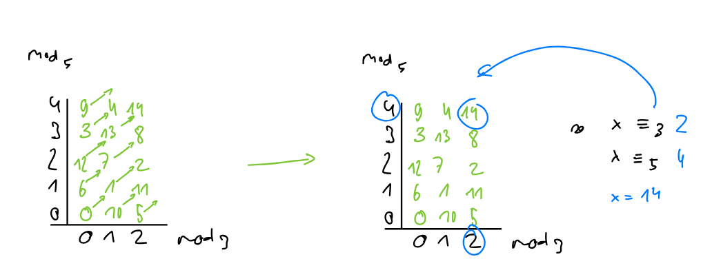
We can also see the CRT as saying that for all $m_1,\dots ,m_r$ pairwise relatively prime, there exists a unique solution $x$ mod $M=m_1\cdot \cdots \cdot m_r$ for the equations.

Or seen still otherwise, there is a unique bijective mapping from the numbers $[0;M-1]\in \mathbb{N}$ to each modulo $m_1,\dots ,m_r$. This mapping can be made visible in such a table:

Technique

The Chinese Remainder Theorem is very useful to make big operations inside an $R_m$ easier to process.

Example: Computing $R_{77}(10^{60})$

$R_{77}(10^{60})$ can be decomposed into two sub-remainders. As $77=7\cdot 11$, we can use: $10^5{\equiv }_7{3}^5{\equiv }_7{2}^3{\equiv }_{7}8{\equiv }_{7}11$ and $10^5{\equiv }_{11}1-1^5{\equiv }_{1}1-1$Thus $1^{60}{\equiv }_{7}1$ and $-1^{60}{\equiv }_{11}11$. Then we have $R_7(10^{60})=1$ and $R_{11}(10^{60})=1$, thus $R_{77}(10^{60})=1$.

General Technique When the final remainders are not both simple values like 1 and 1, you need to find $x$ such that:

• $x\equiv a(\mathrm{mod}{m}_1)$
• $x\equiv b(\mathrm{mod}{m}_2)$ where $\gcd (m_1,m_2)=1$.

Solution: Use the formula $x{\equiv }_{M}a\cdot m_2\cdot (m_2^{-1}\mathrm{mod}{m}_1)+b\cdot m_1\cdot (m_1^{-1}\mathrm{mod}{m}_2)$ where $M=m_1\cdot m_2$ (for the specific case of a decomposition into two formulas).

Brief Example: If $R_7(n)=3$ and $R_{11}(n)=5$, then:

• Find $11^{-1}(\mathrm{mod}7)=2$ (since $11\cdot 2=22\equiv 1(\mathrm{mod}7)$)
• Find $7^{-1}(\mathrm{mod}11)=8$ (since $7\cdot 8=56\equiv 1(\mathrm{mod}11)$)
• Calculate: $x=3\cdot 11\cdot 2+5\cdot 7\cdot 8=66+280=346\equiv 38(\mathrm{mod}77)$
• Therefore $R_{77}(n)=38$

Diffie-Hellman Key-Exchange

The Diffie-Hellman key exchange protocol is used to establish a shared key over an insecure channel.

Because modular exponentiation is hard to invert (we basically need to try all possible numbers), we can safely share the $y_B$ and know that an attacker would never be able to figure out the $x_B$ from that.

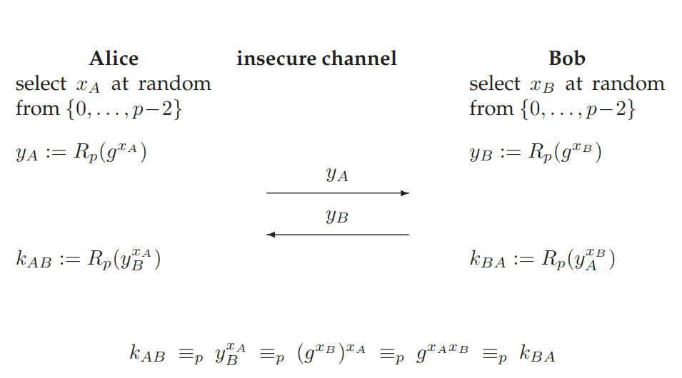
Example Calculation: We use $p=13$ and $g=2$, which are public.

• In private Alice and Bob each select a random element from ${\mathbb{Z}}_p$ that is not $p-1$ (i.e. the inverse).
  • Alice $a=5$, Bob $b=8$
  • Then $A=2^5\mathrm{mod}13=6$
  • Then $B=2^8\mathrm{mod}13=9$
• The secret key is then $S=9^5\mathrm{mod}13=3=6^8\mathrm{mod}13=S$. Thus both are left with the same key. The attacker Eve would have to solve the Discrete Logarithm problem to recover each participants choice of key.

Exercises

Reducing expressions like $R_{11}(9^{2024})$

As $9^{10}{\equiv }_{11}1$, we can reduce the exponent modulo $10$ (see Lagrange’s theorem in chapter 5). Thus $R_{11}(9^{2024})=R_{11}(9^4)=R_{11}(-2^4)=5$.

For this to work however, we need the number and the order of the group (modulo remainder) to be coprime, i.e. $\gcd (9,11)=1$.