Invariants are a concept used to prove the correctness of an algorithm. By proving that the invariant holds for each iteration of the loop, we can prove that the invariant holds at the end of the algorithm. It works similarly to induction.
Search Algorithms
No search algorithm can be faster than because that is the minimum amount of comparisons required to have “seen” all elements.
Linear Search
Linear search simply goes through the entire list and compares the current element to the one we are searching.
The runtime is , as it’s a single for loop.
Linear search does not require a sorted array, it will perform the same on any array.
Binary Search
For binary search, we require a sorted array.
You start in the middle and if the middle element is not the one you’re searching, you recurse on the left OR right side (depending on the middle elements size).
The runtime of binary search is optimal, it is .
# Iterative implementation
def binary_search(arr[0..n-1], x):
	low = 0
	high = n - 1

	while low <= high:
		mid = (low + high) // 2 # floor of the middle element

		if arr[mid] == x:
			return mid
		else if arr[mid] < x:
			low = mid + 1 # set the search bound to be the upper half
		else:
			high = mid - 1 # set the search bound to be the lower half

	return -1
Intuition
Use lo < r as the universal template — it converges to a single index (lo == hi at the end), which is exactly what you want for “find the first/last element satisfying X.”
When to use
lo <= hi?Only for the simple “find exact target, return if missing” case. It gets messy for boundary searches. Stick with
lo < hifor everything.
Template:
int lo = 0, hi = n; // hi = n, NOT n-1 (answer could be "past the end")
while (lo < hi) {
    int mid = lo + (hi - lo) / 2;
    if (condition(mid)) hi = mid;   // mid might be the answer, keep it
    else lo = mid + 1;              // mid is definitely not the answer, skip it
}
return lo; // lo == hi == first index where condition is true
Invariant: the answer is always in . The loop shrinks this to a single point.
-
Why
hi = midbutlo = mid + 1? When condition is true,midcould be the answer (maybe there’s an earlier one), so you keep it. When it’s false,midis definitely wrong, so you skip past it. This asymmetry also prevents infinite loops — the interval always shrinks. -
Why
hi = n? Because the answer might be “no element satisfies the condition,” in which case you want to return (past the end).
Why this works?
Think of condition(mid) as painting the array:
You’re finding the first true. That’s it. Every binary search problem reduces to “find the boundary between false and true in a monotonic boolean array.”
Four Variants:
Just swap the condition:
| You want | Condition | Return |
|---|---|---|
| First target (lower_bound) | a[mid] >= target | lo |
| First target (upper_bound) | a[mid] > target | lo |
| Last target | a[mid] > target | lo - 1 |
| Last target | a[mid] >= target | lo - 1 |
The trick for “last” variants: find the first element that’s too big, then step back one.
Exact match: run lower_bound, then check lo < n && a[lo] == target.
Examples:
// Find target (returns index or -1)
int lo = 0, hi = a.length;
while (lo < hi) {
    int mid = lo + (hi - lo) / 2;
    if (a[mid] >= target) hi = mid;
    else lo = mid + 1;
}
return (lo < a.length && a[lo] == target) ? lo : -1;

// Smallest element > target
int lo = 0, hi = a.length;
while (lo < hi) {
    int mid = lo + (hi - lo) / 2;
    if (a[mid] > target) hi = mid;
    else lo = mid + 1;
}
// lo == a.length means nothing is bigger
lo = midvs.hi = mid
- If we have
lo = midforcond() == true, we need to calculate mid usingmid = lo + (hi - lo + 1) / 2, otherwise we get stuck.- If we have
hi = midwe need the lower half, somid = lo + (hi - lo) / 2.
Using l <= h vs l < h
When we try to find the first occurrence of T in our condition(mid) array, we can either use:
while (l <= r) {
	if (cond(mid) <= target) hi = mid;
	else lo = mid + 1;
}
or
while (l < r) {
	if (cond(mid) <= target) hi = mid - 1;
	else lo = mid + 1;
}
The second one is much faster in practice. It works because when we “overshoot it” by doing hi = mid - 1 when mid is the answer, we get l > r and return l. l is the last known good.
Sorting Algorithms
The lowest time complexity any comparison based sorting algorithm could ever have is !.
We know the following sorting algorithms and their runtimes:
| Algorithm | Runtime (best-case) | Runtime (worst-case) |
|---|---|---|
| Bubble Sort | ||
| Selection Sort | ||
| Insertion Sort | ||
| Merge Sort | ||
| Quicksort | ||
| Heapsort |
You need to know how each of them works, but only need to know how to implement one of the algorithms for the exam.
Note that there are two special cases:
- Bubble sort is best case if we are checking for changes
- Insertion Sort can be in the best case if we don’t use binary search.
But as defined in the lecture, these are the runtimes.
Bubble Sort
Attributes:
- In place
- Best Case:
- Worst Case:
Invariant “Nach Durchläufen der äusseren Schleife sind die grössten Elemente am richtigen Ort.”
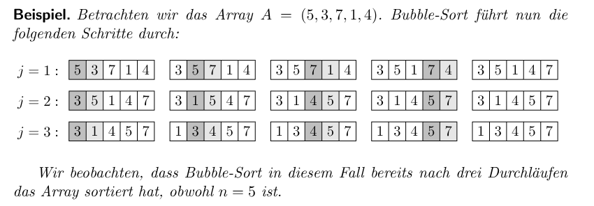
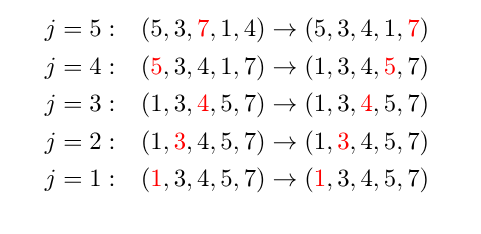
Bubble sort is the easiest algorithm to understand.
It goes through the array times, each time “bubbling up” the biggest element to the end, by swapping.
def bubble_sort(arr[0..n]):
	for i = 0 to n-1:
		for j = 0 to n-1-i:
			if arr[j] > arr[j + 1]:
				swap(arr[j], arr[j + 1])
During each inner iteration, high elements are swapped with their right neighbours until they hit a higher one. The algorithm then continues after that.
We use comparisons and switches.
The worst-case is performance, for an array sorted in descending order.
Selection Sort
Attributes:
- In place
- Best Case:
- Worst Case:
Invariant “Nach Durchläufen der äusseren Schleife sind die grössten Elemente am richtigen Ort.” (Same as for Bubblesort).
Every iteration, selection sort goes through the “unsorted part” of the array, searches for the biggest element and puts it at the end.
def selection_sort(arr[0..n]):
	for i = 0 to n-1:
		max = MIN_VALUE
		max_index = -1

		for j = 0 to n-1-i:
			if arr[j] > max:
				max = arr[j]
				max_index = j

		tmp = arr[n-1-i]
		arr[n-1-i] = arr[max_index]
		arr[max_index] = tmp
Thus on the right-side (or left-side if inverted), we have a list of sorted integers slowly growing, while we only compare the unsorted ones to findest the next biggest to put at the beginning of the sorted list.
Insertion Sort
Attributes:
- In place
- Best Case: (as we use binary search to find the insertion point, as defined in the lecture)
- Worst Case: (reverse sorted array leads to swaps necessary)
Invariant “Nach Durchläufen der äusseren Schleife ist das Teilarray sortiert (es enthält aber nicht zwangsläufig die kleinsten Elemente des Arrays).”
For insertion sort, we start at the left-side and create our sorted array there. We take the next element from the unsorted ones and insert it at the correct place in our sorted array.
This insertion is not constant time! We have to swap it with each previous element!
def insertion_sort(arr[0..n]):
	for i = 1 to n:
		insertion_index = binary_search(arr, arr[i], from index 0 to 1 in arr)
		tmp1 = arr[i]
		arr[insertion_index] = arr[i]

		# Shift the entire array one to the right after the insertion index
		for j = insertion_index+1 to i:
			tmp2 = arr[j]
			arr[j] = tmp1
tmp1 = tmp2Insertion sort is slowly sorting in the elements from the right side into the left side sorted array.
Merge Sort
Attributes:
- not in place, thus the space complexity is . It can be programmed to be in place though.
- Best Case:
- Worst Case:
Invariant Merge sort always sorts correctly when called for a sub-array shorter than . This means that merge has to correctly merge the two sub-arrays into a complete array.
We implement merge sort recursively as follows:
def merge_sort(arr, l, r):
	if l < r:
		mid = (l + r) / 2

		merge_sort(arr, l, mid) # merge sort left
		merge_sort(arr, mid+1, r) # merge sort the right

		arr = merge(arr, l, mid, r) # merge them

# Merge together the two arrays left and right
def merge(arr, l, mid, r):
	# new array
	B = [] of length r - l + 1

	i = l
	j = mid + 1
	k = 0

	# go through the merge left and right, taking the smaller of them to create a sorted merged
	while i <= mid && j <= r:
		if arr[i] <= arr[j]:
			B[k] = arr[i]
			i++
		else:
			B[k] = arr[j]
			j++

		k++

	# append what's left immediately
	while i <= mid:
		B[k] = arr[i]
		i++
		k++

	# append what's left immediately (only one of the loops will actually do something, the other will already have been merged in)
	while j <= r:
		B[k] = arr[j]
		j++
		k++

	return B
Merge sort works by divide-and-conquering the array into smaller chunks. it then merges them together slowly.
The merging works by having two indices showing the current position in the left and right array that we are merging.
We then compare the elements at the indices and take the smaller one. We then increase the counter on that array, while the other stays the same.
As soon as one array has been merged in completely, we can just append the second one (as it’s already sorted).
The worst-case scenario for Mergesort is an array that has alternating small and big elements, thus they will always have to be compared during the merge.
Quicksort
Attributes:
- Not in place (but can be implemented)
- Best Case:
- Worst Case:
Invariant “Elemente links des pivots sind kleiner und Elemente rechts des Pivots sind größer als das Pivot-Element selbst.”
Quicksort works by taking an element as the “pivot”. We then split the array in to two parts: one smaller than the pivot and the other bigger.
We then swap the pivot into the middle of that.
Repeat for each of the smaller subdivisions, until you arrive at single-array elements.
We usually choose the last element (element r) as the pivot, which can go wrong if the array is already sorted. Then we only have split the array into one part, with size . In the best case the pivot is exactly in the middle and we can perfectly recurse with .
def quicksort(arr[1..n], l, r):
	if l < r:
		k = split(arr, l, r)

		quicksort(a, l, k-1)
		quicksort(a, k+1, r)

def split(arr[1..n], l, r):
	p = arr[r] # the pivot element on the right
	k = count_smaller(arr, p)

	B = [] * (r - l + 1) # new array for storage

	i = l
	j = k + 1

	for s in range(l, r):
		if arr[s] <= p:
			B[i] = arr[s]
			i += 1
		else:
			B[j] = arr[s]
			j += 1

	copy(B, arr[l, r]) # copy the B array into the subset of arr
The worst-case is if we have an array that is already sorted. If we instead randomly choose the pivot, we avoid the worst-case pitfalls.
Heapsort
Attributes:
- Is in place, we simply reuse the old-arrays memory space to create a heap
- Best Case:
- Worst Case:
Invariant The heap property is correct for the maxHeap. Then the biggest element will always be on top.
Heapsort works like selection sort by always selecting the largest element and placing it at the end of the sorted array, but instead of having to do an expensive linear search for the largest element, we make it .
This is done by converting the array into a MaxHeap before sorting. This Heap is a tree that has the property that children are always smaller than their parents.
def heapsort(arr[1..n]):
	H = heapify(arr)

	for i in range(n, 1):
		A[i] = extract_max(H)
Extract Max
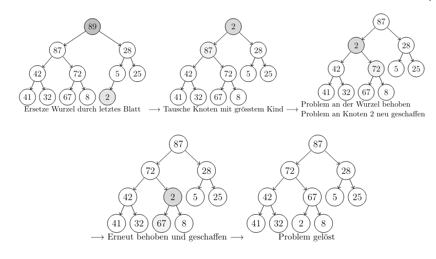
The extract max operation works by taking the root node, the biggest element in the heap by it’s definition and restoring the heap condition. We remove the root and replace it by the element that is most to the right (last element in the array storing the heap).
Then we “versickern” this small element, until the heap condition is restored. We swap it with the larger of the child nodes, until it’s bigger than both of it’s children. This takes time as the tree has maximum levels.
Creating the Heap
Note the property that the children of a node k in a tree are at 2k and 2k + 1. This means that the tree is stored in memory by levels.
To create the heap, we define an insert function and then use it to insert the elements in order of their appearance in the original array.
This works by inserting the node at the next free space in the tree, i.e. first to the left, then right (to conserve the tree structure).
Then we restore the heap condition by reverse-”versickern” the element until it’s restored. You swap it with it’s parent nodes until the condition is restored.
How fast can we sort
There is a lower bound for the worst-case of a comparison based sorting algorithm, which is .
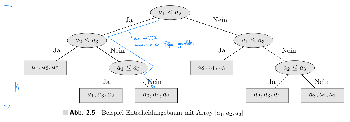
The proof is as follows:
- the algorithm has to correctly sort all arrays, thus every permutation of an array.
- We create a decision tree where each leaf is one permutation, while each node is a comparison of elements, which lead to the correct permutations.
- In the worst-case, an algorithm has to therefore execute comparisons, where is the height of the tree.
- The height of such a tree is permutations .
- Since a comparison is constant time, we need comparisons.
There are non-comparison based sorting algorithms, for example Bucketsort.