DP is working on a similar idea to proving that algorithms work by using an invariant and showing it holds over the course of the execution.
In DP, we have an invariant that shows us how to calculate the solution for smaller problems.
This allows us to then write recursive or bottom-up algorithms that find solutions to our Gesamtproblem.
Memoization and Bottom-Up
Naive implementation of Fibonacci:
def fib(n):
	if n <= 2: return 1 # recursion stop

	return fib(n-1) + fib(n-2)
This implementation is correct, it doesn’t run very fast though. We have seen in the Übungen that this has exponential runtime of .
There are two approaches that allow us to do better!
Memoization
Memoization uses the storage of intermediate results to prevent us from having to re-calculate them at every turn.
We store an array memo[1, ..., n] which contains the results of the computation for each index. This can then be used to do the following:
memo[1] = 1
memo[2] = 1

def fib(n):
	if memo[n] != -1: return memo
	return fib(n-1) + fib(n-2)
This will massively speed up computation, to , as each value now only has to be computed once. Accessing array elements here is .
Bottom Up calculation
We can also go from the other way around, computing them in increasing order.
F[1..n] # new array
F[1] = 1
F[2] = 1
for i in range(3, n):
	F[i] = F[i - 1] + F[i - 2]
Bottom-Up vs. Memoization
Recursion:
- Memoization is often easier to implement using recursion
- Recursion is easier to read
- we don’t need to explicitly think about the order we compute the values in
Bottom-Up:
- more efficient as not stack heavy (no stack limits either)
- memory optimisations are possible by keeping only one row of a DP-table for example
Core of DP
We need to find a fitting subproblem that is easier to solve. This subproblem will often call upon earlier results recursively. We can then solve these problems and construct the solution from them.
We need to explicitly write a recursive formulation of the problem, which requires us to think about base cases!
We then need to think about how to compute the solutions to the subproblems, in which order and using recursion or bottom-up. We then need to define how to extract the final solution.
Finally we can calculate the run-time, for which the size of the DP-table is very useful. Usually the elements in there can be calculated in constant time, which means the total runtime is the size of the table.
Maximum Subarray Sum
Subarray vs. Subsequence vs. Subset
There is an important differentiation to be made between the different problems to do with sub-…:
- A subarray is a continous partition of the original input array
- A subsequence is a non-continous partition of the original input array that preserve the order.
- A subset is any subset of the elements of the original array.
Essentials
- Runtime
- DP-Table
DP[1..n]
Recursion:
Base Case:
Algorithm
def MSS(A[0..n - 1])
	R = A[0]
	RM = A[0]
	for j = 1 to n-1:
		R = max(A[j], R + A[j])
		RM = max(RM, R)
	return RM
Description
We want to find the subarray that maximises the sum in an array of integers. Formally we want to find and such that with such that is maximal, where the empty array is also valid.
Subproblem: We define the randmax as the maximum subarray sum ending in :
As the either contains only or it contains another maximum subarray sum ending in , we can define:
The base case is .
To extract the solution we can take the maximum in our DP-table and otherwise 0 if they are all negative.
As calculating each cell of the DP-table takes time (it’s only a single comparison and array access), the final runtime is .
Jump Game
Essentials
- Runtime for the optimised one ( for naive approach).
- DP-Table
DP[0..k]orDP[1..n].
Recursion:
Base Cases: ,
Algorithm :
def MinJumps(A[0..n-1]):
	dp[0] = 0
	dp[1] = A[0]

	k = 1
	while dp[k] < n-1:
		k = k + 1
		dp[k] = -infinity

		for i = dp[k-2] + 1 to dp[k-1]:
			dp[k] = max(dp[k], i + A[i])

	return k
Description
We need to find the minimal amount of jumps needed to get from the beginning of the array to the end. From position we can jump to and . We start at . All numbers in the array are natural numbers .
We can therefore always jump at least , thus the maximum is jumps.
Two different approaches
We define our problem as . The final solution is then simply . The recursive equation is
We find the cell in the array that leads to our current position with the fewest jumps.
We can also use a different approach by switching our variables. This approach often works in DP problems (Knapsack also).
Instead of thinking in array cells, we think in cells we can reach in jumps. We switch and , making our DP-table . The solution is then the smallest for which .
We get the following recursive equation
We have . The positions reachable in jumps are . Thus we search the maximum position reachable from those by looking for the highest .
We can further optimise this by seeing that we only need to look at as we can reach with jumps already. Thus our recursion becomes
And base cases and . As each now only contributes to a single maximum, we have a runtime of . This is because after we have once, the next steps will not go below that threshold.
Lower bound: We can see that is optimal as we have to look at each element at least once. Otherwise we could have where if we dont look at we will not find the optimal number of jumps.
Longest Common Subsequence (Längste Gemeinsame Teilfolge)
Essentials
- Runtime: (can be improved to or )
- We can also reach for the case
- DP-Table:
DP[0..n][0..m]for lengths of the strings
Recursion:
Base Cases:
Algorithm
def LCS(X[1..m], Y[1..n]):
	for i = 0..m: L[i,0] = 0
	for j = 0..n: L[0,j] = 0

	for i = 1..m:
		for j = 1..n:
			if X[i] == Y[j]:
				L[i,j] = L[i-1,j-1] + 1
			else:
				L[i,j] = max(L[i-1,j], L[i,j-1])
	return L[m,n]
Description
We want to find the longest common subsequence that two strings share. For example TIGER and ZIEGE share IGE as a LGT.
We have
The length of the LGT is then simply .
We compute the LGT by distinction between three cases:
- as for two empty strings we have an empty LGT
- for and :
- In this case as the last element in our LGT. The rest of the LGT must then be an LGT of and .
- This choice of last element is as good as any other, it leaves more choice for the LGT from the previous elements.
- and :
- In this case, this cannot be the last element of the LGT, thus it’s either an LGT of and OR and .
This gives us the following recursion:
We can calculate this value bottom-up by first going row-wise left to right or column-wise top to bottom. Then we never need an element not yet calculated.
Backtracking
We can find the actual LGT itself by using backtracking on the DP-table.
![]()
If we go diagonally, it’s because the elements were the same. Thus that element is part of the LGT. If we went horizontally, then it was not part of it.
Editing Distance
Essentials
Recursion:
Base Cases: ,
Algorithm:
def EditDistance(X[1..m], Y[1..n]):
	for i = 0..m: D[i,0] = i
	for j = 0..n: D[0,j] = j
	for i = 1..m:
		for j = 1..n:
			cost = 0 if X[i] == Y[j] else 1
			D[i,j] = min(
				D[i-1,j] + 1, # delete
				D[i,j-1] + 1, # insert
				D[i-1,j-1] + cost # replace
			)
	return D[m,n]
Description
The editing distance of two strings is the minimum amount of edits (insert, delete, replace) we need to perform in order to transition one into the other. We can use the LGT to calculate the editing distance.
The editing distance of TIGER to ZIEGE is as we replace T by Z, then remove R and insert E. There are of course other ways to do this, but they can’t be shorter.
We track the character through the process of finding the for two strings and :
- is deleted at some point, thus , i.e. searching for the ED between the strings and the same b.
- A crucial insight is that if a character is deleted, it doesn’t matter when in the process it is done so.
- is not deleted and ends up somewhere in .
- In this case no character can be behind (it would cost an extra op to delete and insert it again), thus we have .
- is not deleted and ends up at
- In this case we can’t insert any other character behind , thus if otherwise .
We can calculate each entry of the DP-Table in constant time , thus the total runtime is .
Backtracking
We can again use the DP-Table to find the edits performed:
![]()
Subset Sum (Teilsummenproblem)
Essentials
- Runtime:
- DP-Table:
DP[0..n][0..b]
Recursion:
Base Cases:
Recursion:
Description
We want to find the subset such that . Such a subset sum must not exist for all obviously.
There is a special version of this problem called the partition problem (Partitionsproblem) which asks if we can divide the numbers of into two subsets with the same sum.
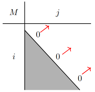
Our sub-problem is
To recursively calculate this value we observe that either is in the subset sum, or we look for a subset sum which includes and thus sums to :
as we can use . for all as we can’t use any elements. We calculate in ascending order of .
To find the subset, we have to include all which have a diagonal increase in the DP-table, as that is the case where we take .
This problem runs in pseudo-polynomial runtime.
Pseudo-Polynomial Runtime
We have . But while is the length of the array, is the value of a user entry.
This means that could be extremely large, while looking like a polynomial factor in our model.
If we chose for example, our runtime would be which is exponential. On the other hand, if is polynomial in relation to , like for , then our total runtime is also polynomial.
Knapsack Problem (Rucksackproblem)
Essentials
- Runtime: or .
Recursion:
Base Cases:
Algorithm:
def Knapsack(v[1..n], w[1..n], W):
	for i = 0..n: dp[i][0] = 0
	for w = 0..W: dp[0][w] = 0
	for i = 1..n:
		for cap = 1..W:
			if w[i] <= cap:
				dp[i][cap] = max(
					dp[i-1][cap],
					dp[i-1][cap - w[i]] + v[i]
				)
			else:
				dp[i][cap] = dp[i-1][cap]
	return dp[n][W]
Description
The knapsack problem asks which items of weight and profit we should take for a weight limit to reach a profit . This is a a subset problem.
A greedy algorithm (chooses local optimum in the hopes of it corresponding to the global optimum) which always takes the most profitable item (or the lightest ones, or the ones with the best profit/weight ratio) will fail, as we can always construct an unfavorable input.
Our subproblem is:
So we either don’t use an item because it busts our limit, or we can use it and take the bigger profits between using it and not.
Backtracking works like usual, if we go diagonally, we took the item, otherwise not.
This algorithm is again pseudo-polynomial as our input is not the length of an array but a user entry.
Alternative: There is also an alternative DP solution, which uses by variable switching. We look for items that give us profit by taking the subset that has minimal weight.
Approximation for the Knapsack Problem
As we don’t expect to find an algorithm to solve the Knapsack problem in polynomial time, we can instead look into finding an algorithm that approximates the solution.
We want to find an algorithm that has polynomial runtime and returns a value close to the actual solution.
To do this, we round the profits and solve the Knapsack problem for these rounded profits:
where K is the multiple that we round to. As we didn’t change the weights and only the profits, our approximated solution is still a valid subset for the original problem
Key Properties:
- The rounded profits satisfy:
- Since we only change profits (not weights), any valid solution for the rounded problem is also valid for the original problem
- We can exclude items with beforehand (they won’t fit anyway)
Performance Analysis
Let:
- = optimal solution for the original problem
- = optimal solution for the rounded problem (what our algorithm computes) - = maximum profit of any item
Key Inequalities:
- (sum of rounded profits in OPT is at least )
- (since OPT has at most items)
Approximation Quality: Through a series of inequalities, we can show:
where denotes the total profit of a solution. To make small relative to , we introduce a parameter and set:
This gives us:
Therefore:
Result: The algorithm achieves a -approximation — the profit of our solution is at least times the optimal profit.
As our new DP table now only has length as we only have to fill every th column in the table. We can choose an arbitrarily big , for a trade off in accuracy.
With :
- Runtime:
- Since , this simplifies to:
Examples:
- For : We get a 90% approximation in time
- For : We get a -approximation in time
Longest Ascending Subsequence (Längste Aufsteigende Teilfolge)
Essentials
- Runtime:
Base Cases:
tails = [a_1] we initialise the array with our first element (it’s the smallest at that point).
Algorithm:
def LAS(A[1..n]):
	tails = [] # tails[l] = kleinstes Endelement einer Folge der Länge l+1
	for x in A:
		pos = binary_search_first_ge(tails, x)
		if pos == len(tails):
			tails.append(x)
		else:
			tails[pos] = x
	return len(tails)
We can use an array for this by just initialising it to length and then setting all values to .
Description
We are given an array of distinct whole numbers. We want to find the longest ascending subsequence of (i.e. the indices for which the longest is strictly ascending).
We define
To calculate these values recursively we distinguish:
- : as the LAT of length 1 always exists
- : iff. there is a such that and . We can then extend this subsequence by .
- otherwise
This is not the most efficient solution however with , as we need to compute go through all previous possibilities.
More efficient
We define a table as the smallest possible ending of a LAT of length in the subarray . If there is none, (no smaller element exists to extend the sequence).
The recursion is defined for the following cases:
- : then if and otherwise
- :
- We do not use , and in this case
- We use . This is only possible if , as only then we can actually append to this longest subsequence. Then
- We therefore need to take the smaller of these two:
- if and , then
As every entry in our table can be computed in constant time, we have a runtime of .
Even more efficient
We can still improve the runtime here by recognising that as we can take any longer subsequence and shorten it by 1. This means that the rows of our DP table are sorted:
By only keeping the latest version, i.e. the smallest element for any , we can have a 1d DP table.
We can always use binary search in our sorted table to find the place where , i.e. the one we need to update.
We return the biggest for which the entry is .
P = NP?
This question asks if the class of problems computable in polynomial time is equal to the class of problems solvable in polynomial time.
Said differently, if we can check a solution in polynomial time, can we also find it?
If we can solve problems like the subset sum or the knapsack problem in polynomial time we have shown that .
Matrix Chain Multiplication (Range DP)
Essentials
- Runtime:
- DP-Table:
DP[1..n][1..n]
Base Case:
Recursion:
Note that the computation order is diagonal here.
Algorithm
def Matrix(k[0..n]):
dp[][] = infinity
for i in [1..n]:
dp[i][i] = 0
for l in [2..n]:
for i in [1..n - l]:
# Set j as the end
j = i + l - 1
dp[i][j] = min([
dp[i][s] +
dp[s + 1, j] +
k[i - 1] * k[s] * k[j]
| for s in [i..j - 1]
])
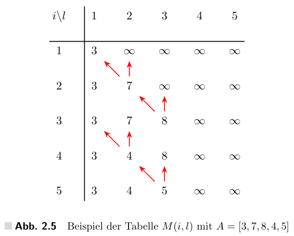
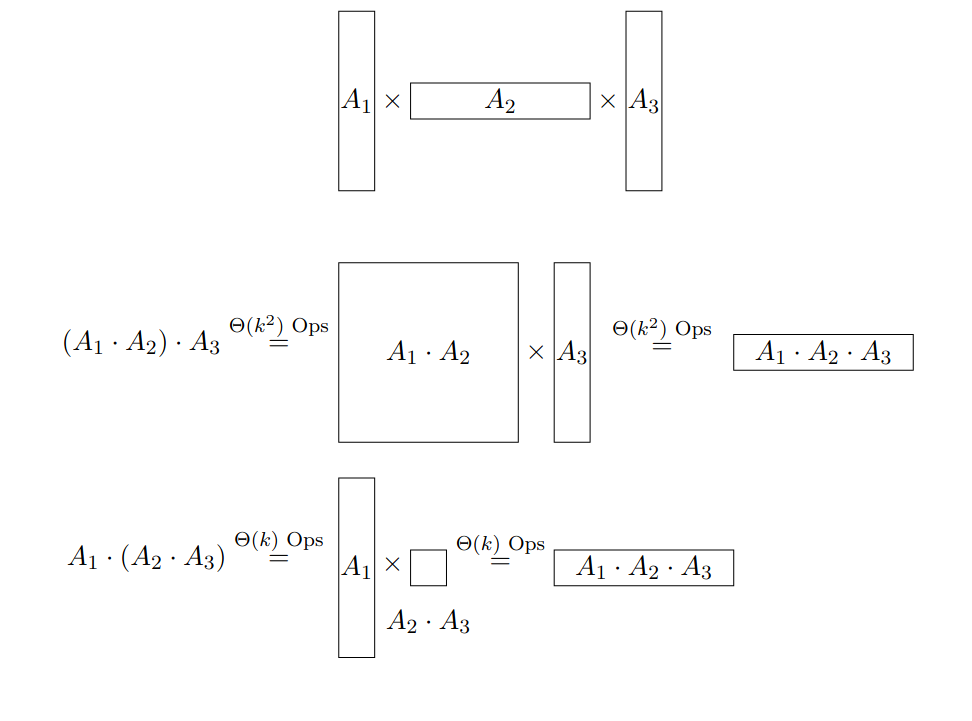
return dp[1][n]Description
For matrices we want to find the multiplication order that requires the least operations. Matrix has entries.
Each entry of our DP table is the minimal number of operations needed to compute the product .
To compute the values recursively, we look at all possible positions , where and “add parentheses” around .
The total number of multiplications needed then is to find multiply the rest and to compute the product of both parts.
- Part 1 has size and the second .
- The resulting matrix has entries
- For each of which we need to compute the scalar product of two long vectors.
This gives us a total of operations.
- For each of which we need to compute the scalar product of two long vectors.
Computation Order: As each entry depends on subarrays of smaller size ( thus and ), we need to compute by increasing length .
Solution Extraction
The solution is .
Runtime
Each entry in our DP table is calculable in as we need to try possible positions for the split .
The total runtime is thus . (By being more precise and summing over we also only get )
Tips for the Exam
DP Table Recursion
A common mistake while establishing the recursion for the DP-Table is to have DP[...][b - A[i]] where b - A[i] goes out of bounds. If we don’t say false if out of bounds, this is a mistake.
DP Table Solution Runtime
- When specifying the runtime of the solution, always specify how long it takes to extract the solution. It’s often .