9. Minimum Spanning Trees

Given a connected, undirected graph $G=(V,E)$ with non-negative edges, an MST (Minimum Spanning Tree) is a subgraph $T=(V,E_T)$ that fulfills the following conditions:

• spanning it connects all vertices (every node is reachable)
• acyclic it’s a tree thus it’s acyclic. If there was a cycle, we could remove the most expensive edge and it would remain an MST
• minimal the sum of the weights in $E_T$ is minimal, i.e. the smallest possible among all spanning trees of $G$.

We can infer from the fact that we want the cost to be minimal, that the number of edges should also be minimal (otherwise we can again remove one). Therefore, the MST has only $|V|-1$ edges.

A safe edge is an edge that has to be included in all MSTs (if the edge-weights are distinct, which means there is one unique MST). Identifying them allows us to iteratively build such a tree.

Restrictions on the Graph for an MST to exist

The graph needs to be connected, otherwise we can only find an MSF, a minimum spanning forest of disconnected trees.

A graph for which we want to find an MST does not need to have positive edge-weights. Even though Prim’s algorithm is similar to Dijkstra’s there’s no restrictions for edge-cost as we don’t use the triangle inequality.

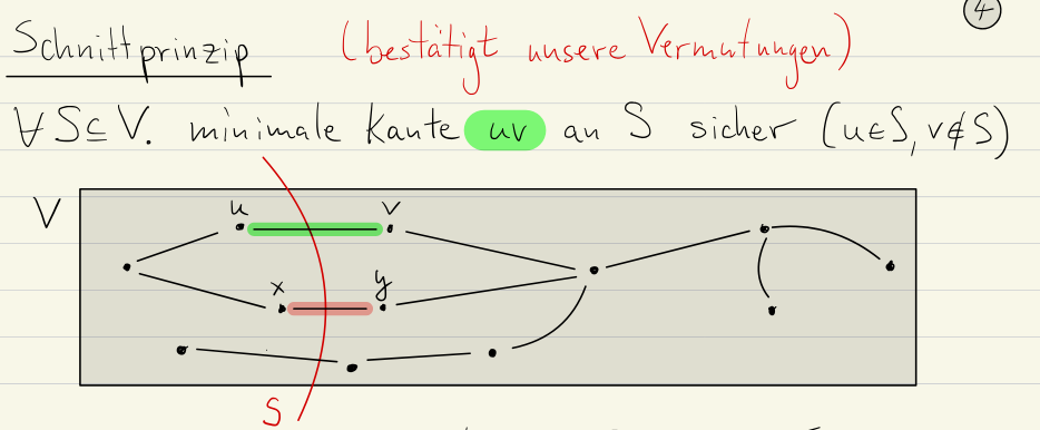
Schnittprinzip (Cut Property)

To join a set of disjoint connected components, we need to use an edge to join two of their vertices. The idea is that the cheapest such edge is always a safe edge.

Proof Idea: If we have an edge $uv$ that joins two connected components and choose edge $xy$ with a higher cost to connect them, by replacing $xy$ through $uv$ we get a cheaper tree, ergo using $xy$ it wasn’t an MST.

A locally minimal edge is an edge that is the cheapest connection between a vertex and any vertex outside it’s immediate neighbourhood. This is the more local version of the Schnittprinzip.

Thus our idea for constructing an MST will be to start with $E_T=\varnothing$ and iteratively add safe edges.

Boruvka’s Algorithm

Runtime: $O((|V|+|E|)\cdot \log |V|)$ Restrictions: undirected, weighted, connected graph Usage: Build an MST

For the correctness of Boruvka, we assume that all edges have distinct weights (in the real world we could use an id or something else to break ties).

1. For Boruvka, we start with the set of edges $F=\varnothing$. We treat each of the isolated vertices of the graph as it’s own connected component.
2. Each vertex marks it’s cheapest outgoing edge as a safe edge (making use of the cut property). We add these to $F$.
   • Note that some of the edges might be chosen by both adjacent vertices, we still only add them once.

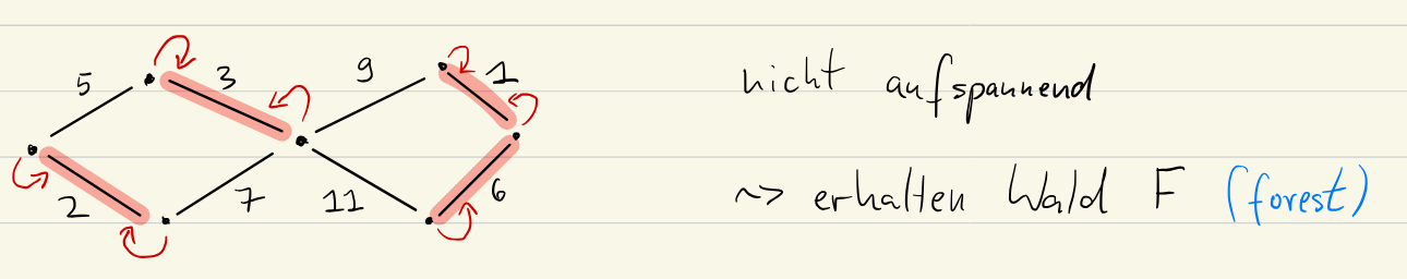
3. Now, repeat by finding the cheapest outgoing edge for each component. Do this until all are connected.
4. $F$ constitutes the edges of the MST.

Code

Boruvka(G):
    F = ∅  # Set of MST edges
    Components = {{v} for v in V} # Initially, each vertex is its own component
 
    while |Components| > 1:
        SafeEdges = ∅
        for each component C in Components:
          cheapestEdge = findCheapestEdge(C, G) # finds the edge with minimum weight connecting C
          # to another component. Returns None if it doesn't exist.
          if cheapestEdge is not None:
            SafeEdges.add(cheapestEdge)
 
        for edge (u,v) in SafeEdges:
            Components = mergeComponents(Components, u, v) # Merges components containing u and v
            if (v,u) not in F: # prevent duplicate edges
                F = F ∪ {(u, v)}
                
    return F

Note that this algorithm is parallelisable.

Runtime

For each iteration, we need to examine all edges to find the cheapest one: $O(|V|+|E|)$ (calculate connected components with DFS: $O(|V|+|E|)$ and then go through each one $O(|E|)$ to find minimal). We iterate a total of ${\log }_2|V|$ times, as each iteration joins at least two halves. Total runtime is $O((|V|+|E|)\cdot \log |V|)$.

We assume efficient datastructures for managing connected components and finding the minimum edges.

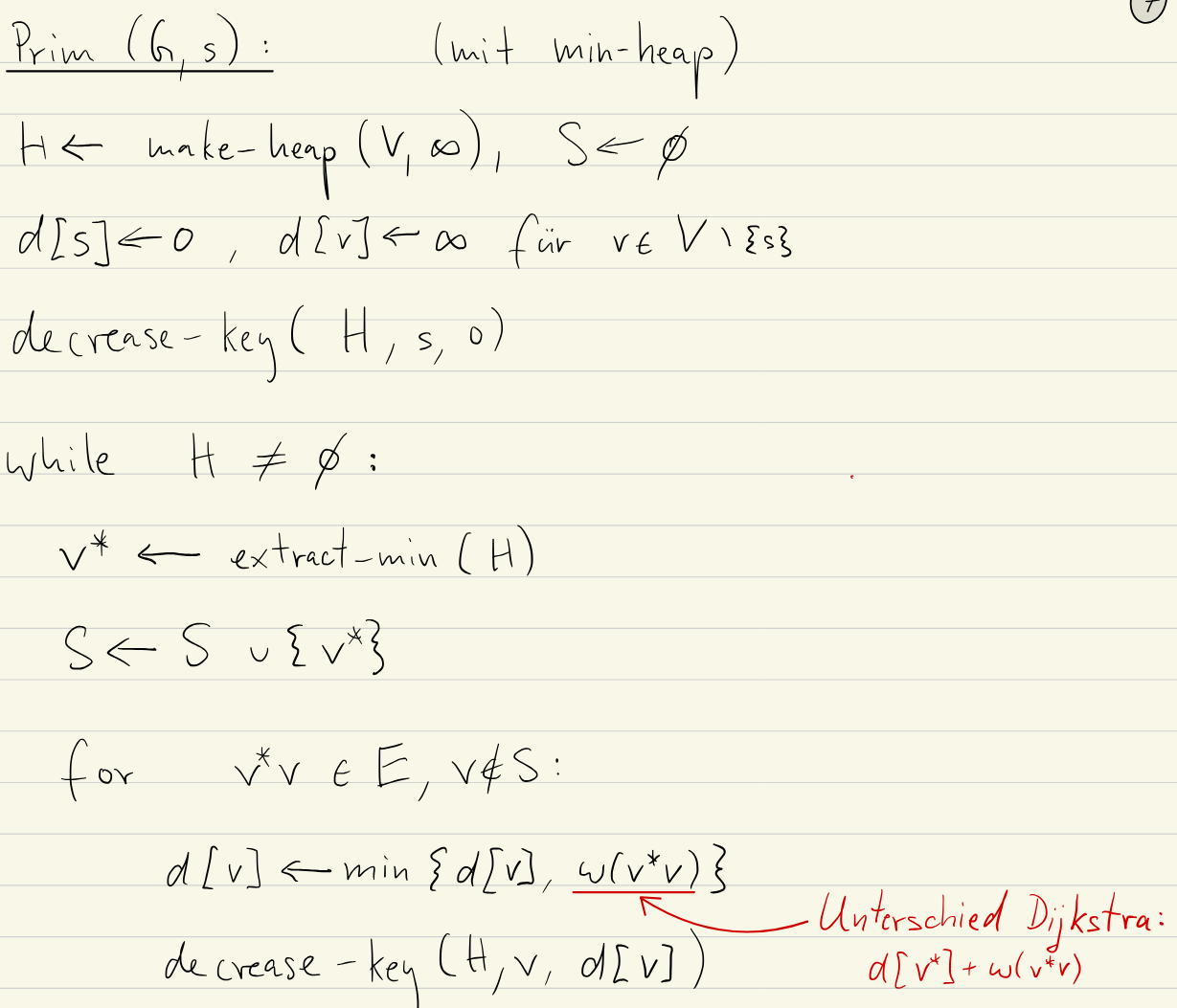
Prim’s Algorithm

Runtime: $O((|V|+|E|)\log |V|)$ Restrictions: undirected, weighted, connected graph Usage: Finding an MST

Prim’s algorithm starts with a single vertex and grows the MST outwards from that seed.

1. Initialisation:
   • Select and arbitrary starting vertex $s$ and empty set $F$
   • Set $S=\{s\}$ tracks the vertices in the MST
   • Each vertex gets a key[v] = representing the cheapest known connection cost to $v$:
     • $\infty$ if no edge connects $s$ to $v$
     • $w(s,v)$ if edge $(s,v)$ exists
   • Use a priority queue $Q$ (Min-Heap) to store the vertices, in order of lowest key cost
2. Iteration:
   • Select and add Extract the vertex $u$ with the minimum key from $Q$. This is the cheapest to connected to the current MST. Add $u$ to $S$.
   • Update Neighbours For each neighbour $v$ of $u$ not in $S$:
     • If $w(u,v)<\text{key}[v]$ update key[v] = w(u, v) and update the priority in $Q$.
       • This discovers potentially cheaper connections to vertices outside the current MST. If a cheaper edge to $v$ is found, the current value in key[v] cannot be part of the MST
3. Termination: When $Q$ is empty, all vertices are in $S$ and connected, and the edges chosen are in the MST (tracked in the set $F$ through updates).

Algorithm

Runtime

Using a binary heap as the priority queue, Prim’s algorithm has a runtime of $O((|V|+|E|)\log |V|)$ (like Dijkstra’s and Boruvka’s).

Invariants holding for Prim’s

The following invariants hold during execution:

1. The priority queue $H=V\setminus S$ ($V$ set of all vertices, $S$ vertices currently in the MST). Priority queue never contains a vertex already in the MST.
2. The distances d[.] = in the distance array are the values of the vertices in the priority queue. (see line decrease_key(H, v, d[v]))
3. $\forall v\notin S,v\ne s$, $d[v]=\min \{w(u,v)|(u,v)\in E,u\in S\}$ ($\infty$ if no such edge exists)

The 3rd invariant $d[v]=\{\begin{array}{ll}0,& \text{if }v=s\text{ (the starting vertex)}\\ {\min }_{(u,v)\in E:u\in S}\{w(u,v)\},& \text{if }v\in V\setminus S\text{ and }\exists (u,v)\in E\text{ with }u\in S\\ \infty ,& \text{if }v\in V\setminus S\text{ and }\nexists (u,v)\in E\text{ with }u\in S\end{array}$ensures that d[v] always reflects the minimum cost to reach vertex v from the current MST.

We always want to add the vertex with the cheapest edge connecting it to the MST, thus this invariant has to hold in order for the algorithm to be correct.

Kruskal’s Algorithm

Runtime: $O(|E|\log |E|+|V|\log |V|)$ Constraints: Undirected, weighted, connected graph (distinct edge weights)

Note that some sources say $O((|E|+|V|)\log |V|)=O(|E|\log |V|)$, as we assume that $|E|\le O(|V{|}^2)$. Use the non-simplified version as in unconnected graphs it might be wrong.

Because the cheapest edge in the entire graph is always a safe edge, Kruskal iteratively builds out the tree from the cheapest edges. We have to be careful not to add edges that would form a cycle as they are not in the MST. Thus Kruskal only considers edges that connect new vertices to the MST.

Algorithm

def kruskal(G):
    F = set()  # Use a set for efficient cycle detection
    for (u, v, weight) in sorted(G.edges(data='weight')): # Access weight data directly
        if find(u) != find(v):
            union(u, v)
            F.add((u, v))
    return F

1. Initialisation: Start with an empty set $F=\varnothing$ to represent the MST edges. Initially each vertex is it’s own seperate ZHK.
2. Iteration:
   1. Sort all edges in the graphs by weight in increasing order.
   2. For each edge $(u,v)$ in sorted order:
      1. If adding $(u,v)$ does not create a cycle (i.e. $u$ and $v$ in different ZHKs)
         1. Add $(u,v)$ to $F$.
         2. Merge the ZHKs of $u$ and $v$

The operation of checking if there is no cycle can be done efficiently using the check of $u$ and $v$ being in different ZHKs. This can be done efficiently using the Union-Find datastructure.

Proof

Induction:

1. BC: After adding 0 edges, each vertex is it’s own ZHK
2. IH: Assume that after adding $k$ edges, $F$ is a subset of some MST
3. IS: Let $(u,v)$ be the $k+1$th edge.
   1. If adding $(u,v)$ creates a cycle, it’s discarded. IH holds.
   2. If there’s no cycle:
      1. $(u,v)$ connects two different ZHKs
      2. As it’s the cheapest, by ordering of edges, that crosses this cut, by the cut-property, it belongs to some MST. Therefore adding it to $F$ maintains the IH.

Runtime

Outer Loop: Kruskal’s iterates at most $|E|$ times: Inner Loop:

• without union-find: checking for cycles requires a graph traversal for each edge, taking $O(|V|)$ per edge for $O(|E||V|)$ total
• With union-find: find and union take an amortised $O(\log |V|)$ per call and over all iterations it takes $O(|V|\log |V|)$ (as union is $O(\log |V|)$ amortised and find is constant)

A dominant factor with union-find becomes edge-sorting, which takes $O(|E|\log |E|)$.

Therefore the overall complexity is $O(|E|\log |E|+|V|\log |V|)$.

Union Find

The Union-Find datastructure provides 3 methods:

1. make(V): creates the DS for $F=\varnothing$
2. same(u, v): tests if $u$ and $v$ are in the same component of $F$
3. union(u, v): merge ZHKs in $F$ of $u$ and $v$ (called when adding the edge from $u$ to $v$)

The DS represents each ZHK using a representative in memory, rep[u]. Each vertex in the same ZHK has the same representative.

1. Then make initialises all $\forall v\in V$, rep[v] = v, this takes $O(|V|)$
2. A same check compares representatives rep[u] == rep[v], this takes $O(1)$

After adding $x$ edges to the forest, the array repr contains exactly $n-x$ different representative values. Each added edge removes one unconnected component.

Merging by iteration

A naive way to merge two ZHKs would be to iterate over all vertices with the same representative and set it to the new one.

# Merge u and v
for x in V:
	if rep[x] == rep[u] # check if x in ZHK of u
		rep[x] = rep[v] # set x to same rep. as v

This takes $O(|V|)$ per merge, which is very inefficient, as it has to be called each iteration.

Merging using membership lists

We introduce members[r], which contains all members of the ZHK with representative r.

# merge u and v
for x in members[r]:
	rep[x] = rep[v]
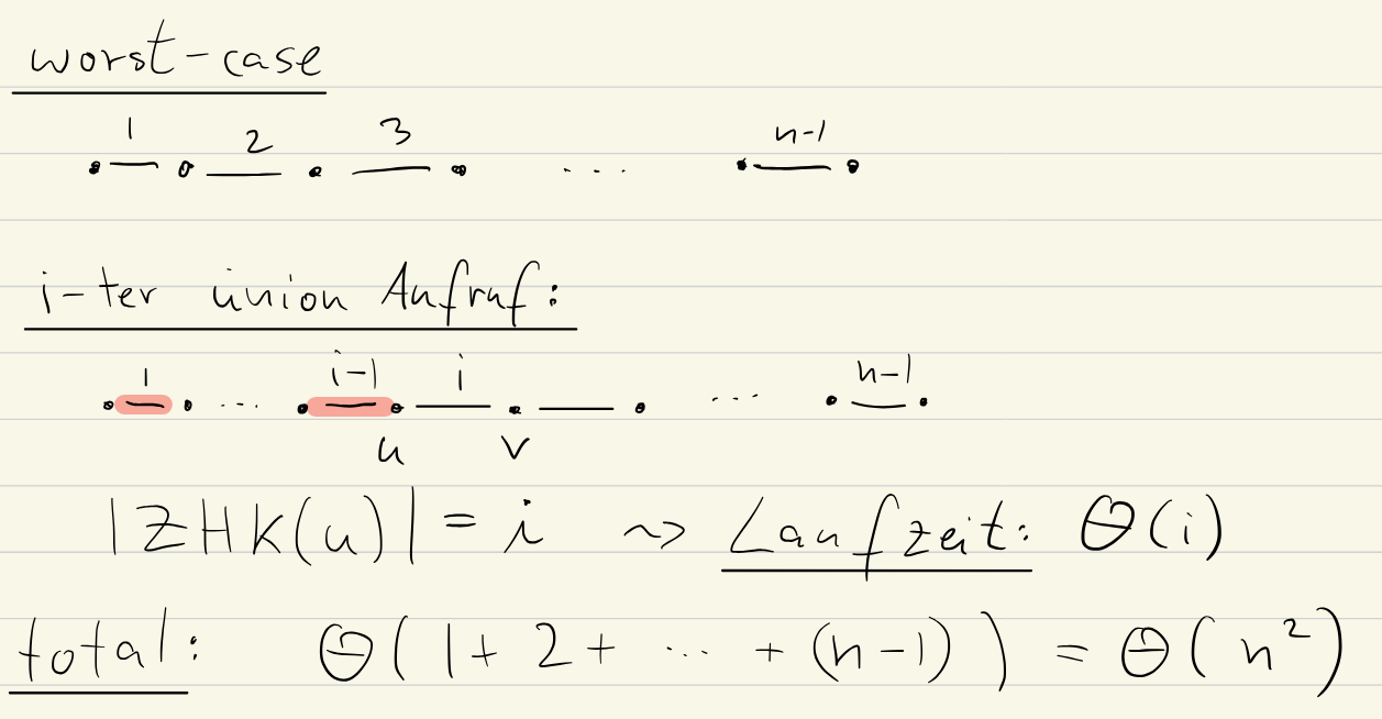
	members[rep[v]] = members[rep[v]] + [x] # add to members of ZHK v

This takes $O(|CON(u)|)$ time (number of members of the ZHK). In the worst case, we take the MST of a “linear” graph, which means we always change $i-1$‘s ZHK in the $i$th iteration.

Merging by rank (members based)

We can improve on this by merging the smaller ZHK into the bigger one. This means that we perform the last updates possible.

By storing rank[r] for each ZHK, we can compare sizes.

if size[rep[u]] < size[rep[v]]:
    for x in members[rep[u]]:
        rep[x] = rep[v]
	members[rep[v]] = members[rep[v]] ∪ {x}
	size[rep[v]] = size[rep[v]] + size[rep[u]]
 
else:
    for x in members[rep[v]]:
        rep[x] = rep[u]
	members[rep[u]] = members[rep[u]] ∪ {x}
	size[rep[u]] = size[rep[u]] + size[rep[v]]
 

Now union takes $\Theta (\min \{|ZHK(u)|,|ZHK(v)|\}$. In the worst case, the minimum is $|V|/2$ as both have the same size.

Therefore over all loops, this would take $O(|V|\log |V|)$ time, as on average we only take $O(\log n)$ time. The graph stays worst case, this is the average of the calls in the worst case.

Proof: We count the number of times rep[u] changes to estimate runtime:

• If rep[u] changes, $|ZHK(u)|\le |ZHK(v)|$
  • thus size of the ZHK of $u$ is always at least doubled.
• As the maximum size of a ZHK is $n$, we need ${\log }_{2}n$ calls.