6. Applications of Orthogonality and Projections

6.1 Least Squares Approximation

One case in which $Ax=b$ usually has no solutions is when trying to fit a line to a set of measurements or datapoints. We can then try to use a least squares approximation to find a best-fitting line.

6.1.1 Minimiser is solution to the normal equations

A minimiser of ${\min }_{\hat{x}\in {\mathbb{R}}^n}||A\hat{x}-b|{|}^2$ is also a solution of $A^{\top }A\hat{x}=A^{\top }b$. When $A$ has independent columns the unique minimiser of $\hat{x}$ is given by $\hat{x}=(A^{\top }A{)}^{-1}{A}^{\top }b$

Notice that $||A\hat{x}-b|{|}^2$ being minimal is equivalent to asking $A\hat{x}$ to be the projection of $b$ onto $C(A)$ (then we minimise $e$ the error). Thus we can solve for $\hat{x}$ (which when multiplied with $A$ gives us the projection) by using the projection, without the final $A$ on the left, which gives us the above equation.

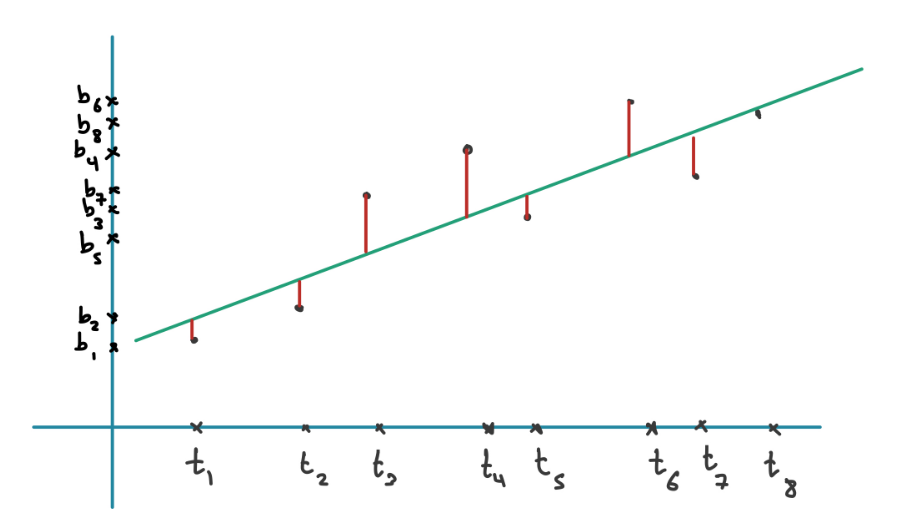
The line here can be represented by the equation $f(x)={\alpha }_{1}x+{\alpha }_0$. We want to find ${\alpha }_0$ and ${\alpha }_1$ that minimise the sum of squares of the error of the fitted line: ${\min }_{{\alpha }_0,{\alpha }_1}{\sum }_{k=1}^m(b_k-[{\alpha }_0+{\alpha }_1{t}_k]{)}^2$ which in Matrix vector notation gives ${\min }_{{\alpha }_0,{\alpha }_1}||b-A\left(\begin{array}{c}{\alpha }_1\\ {\alpha }_0\end{array}\right)|{|}^2$ where $b=\left(\begin{array}{c}{b}_1\\ b_2\\ ⋮\\ b_m\end{array}\right)$ and $A=\left[\begin{array}{cc}1& t_1\\ 1& t_2\\ ⋮& ⋮\\ 1& t_{m-1}\\ 1& t_m\end{array}\right]$

6.1.2 Independent columns of $A$

The columns of the $m\times 2$ matrix defined before are linearly dependent if and only if $t_i=t_j$ for all $i\ne j$.

As all datapoints are unique in time (can’t have two points at one time) this always holds.

6.1.3

If the columns of $A$ are pairwise orthogonal, we get $A^{\top }A$ a diagonal matrix which is very easy to invert. We can convert any $A$ to have orthogonal columns by making sure that the sum of all the $t_k=0$, which can be achieved by shifting the graph on the x-axis.

We can also try to fit any other equation, not just a line here. A parabola could be used by adding a third column to $A$ which contains $t^2$ and adding ${\alpha }_2$.

6.2 The set of all solutions to a system of linear equations

We know that $\forall x\in {\mathbb{R}}^n$, there exist $x_0\in N(A)$ and $x_1\in R(A)$ such that $x=x_0+x_1$ and $x_1^{\top }{x}_0=0$ as $N(A)=C(A^{\top }{)}^{\perp }$ are orthogonal complements.

6.2.1 Unique solutions

Let $A\in {\mathbb{R}}^{m\times n}$. Let $x,y\in C(A^{\top })$. We have that $Ax=Ay\iff x=y$

Proof This is because $x,y$ have unique decompositions into the two fundamental subspaces. $Ax=Ay\iff x-y\in N(A)\iff x^{\top }(x-y)=0=y^{\top }(x-y)\iff (x-y{)}^{\top }(x-y)=0$ and from this follows that $||x-y|{|}^2=0⟹x-y=0$.

6.2.2 Unique solution to a system

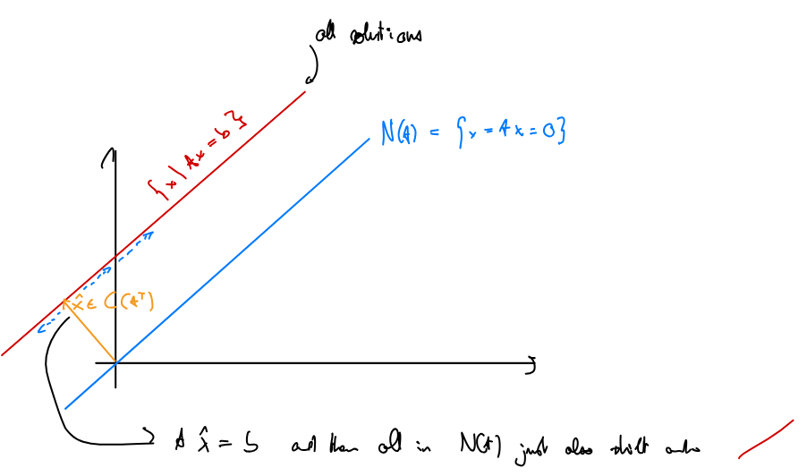
Suppose that $\{x\in {\mathbb{R}}^n|Ax=b\}\ne \varnothing$. Then $\{x\in {\mathbb{R}}^n|Ax=b\}=x_1+N(A)$ where $x_1\in R(A)$ is unique such that $A{x}_1=b$.

This means that if there’s more than one solution to the system (i.e. the nullspace is not $=\{0\}$), then the set of all solutions is a specific solution + the entire nullspace.

6.2.3 Unique in $C(A^{\top }A)$

Suppose that $\{x\in {\mathbb{R}}^n|Ax=b\}\ne \varnothing$. Then there exists a unique vector $x_1\in C(A^{\top }A)$ such that $A{x}_1=b$

The empty solution

We now only need to analyse the case where the given system of linear equations has no solutions: $\{x\in {\mathbb{R}}^n|Ax=b\}=\varnothing$.

This is difficult as proving a negative in this case means exhausting the entire search space (which is infinite) or proving it by using something smarter.

We can issue a “certificate” which proves that a system has no solution.

6.2.4 Proving no solutions

$\{x\in {\mathbb{R}}^n|Ax=b\}=\varnothing ⟺\{z\in {\mathbb{R}}^m|A^{\top }z=0,b^{\top }z=1\}\ne \varnothing$ Note that we don’t need it to be $1$, it just has to be $\ne 0$.

In words: our LSE $Ax=b$ does not have any solutions if and only if there exists a vector $z$ that is orthogonal to all columns of $A$ but not orthogonal to $b$.

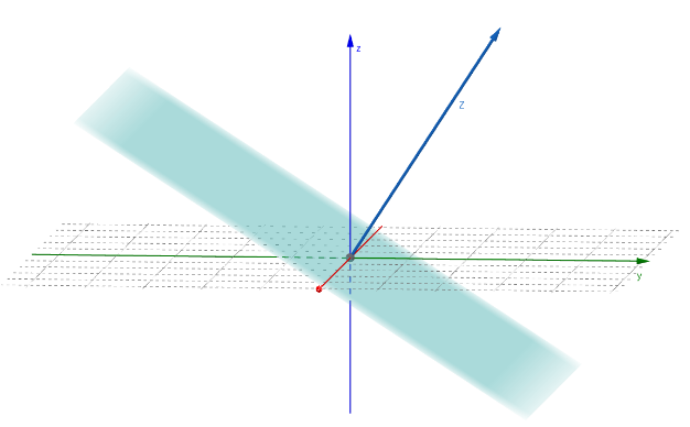
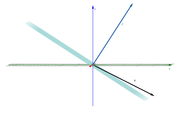
The blue vector $z$ is orthogonal to all in $C(A)$, the blue subspace. If $b$ is not orthogonal to $z$, this means that it cannot possibly be in the subspace, it must be slightly above/below it. Therefore $b\notin C(A)$ and thus there’s no solution.

Proof:

• Verify that $P\ne \varnothing \wedge D\ne \varnothing$ is impossible:
  • If $x\in P$ and $z\in D$ then $0=0^{\top }x=z^{\top }Ax=z^{\top }b=1$
• We now want to show that if $P=\varnothing ⟹D\ne \varnothing$:
  • $P=\varnothing ⟹b\notin C(A)$ (there are no solutions) $⟺b-{\text{proj}}_{C(A)}(b)\ne 0$ (there is an error, $e=b-{\text{proj}}_{C(A)}\in N(A^{\top })$
    • Thus $e\ne 0$ and $z:=\frac{1}{e^{\top }e}e$
    • $z\in N(A^{\top })⟹A^{\top }z=0$
    • $b^{\top }z=\frac{1}{e^{\top }e}{e}^{\top }b=\frac{1}{e^{\top }e}{b}^{\top }e$ but we can rewrite $b=(p+e)$ and thus $b^{\top }z=\frac{1}{e^{\top }e}{p}^{\top }e+\frac{1}{e^{\top }e}{e}^{\top }e$
      • we know the first term is $0$ as $p^{\top }e=0$ as they are in orthogonal subspaces
      • the second term is $1$ as it’s $\frac{e^{\top }e}{e^{\top }e}$.
  • Thus $z\in D$

Example:

• $P=\{x\in {\mathbb{R}}^3|x_1+2x_2-x_3=1,2x_1+4x_2-2x_3=0\}$
• The system $D=\{z\in {\mathbb{R}}^m|A^{\top }z=0,b^{\top }z=1\}$ is then $$ D = { z \in \mathbb{R}^2 \ | \ z_1 + 2z_2 = 0, 2z_1 + 4z_2 = 0, -z_1 - 2z_2 = 0, z_1 = 1 } $$$P = \emptyset$and$D \neq \emptyset$because$z = (1, -\frac{1}{2})^\top \in D$.

Applications:

1. If our matrix $A\in {\mathbb{R}}^{m\times n}$ had linearly independent rows, then there would be solutions for all points in $b\in {\mathbb{R}}^m$. Since the rows are linearly independent, the only solution to $z^{\top }A=0$ is $z=0$. Hence $z^{\top }b=0\ne 1$. Thus there is always a solution for the $P$.
2. We can also show that a vector $b$ is linearly independent from a set of vectors $a_1,\dots ,a_n$. We just put them into the matrix equation $Ax=b$. If there is no solution, $b$ is independent. But to show the system has no solutions, we need our new formula.

6.3 Orthonormal Bases and Gram-Schmidt

6.3.1 Orthonormal vectors

Vectors $q_1,\dots ,q_n\in {\mathbb{R}}^m$ are orthonormal if they are orthogonal and have norm $1$. In other words, for all $i,j\in \{1,\dots ,n\}$ $q_i^{\top }{q}_j={\delta }_{ij}$where ${\delta }_{ij}$ is the Kronecker delta (${\delta }_{ij}=0\text{if }i\ne j\text{ and }1\text{ if }i=j$).

Thus all vectors are pairwise orthogonal $q_i^{\top }{q}_j=0$ and all of them have norm $1$: $q^{\top }q=||q|{|}^2=||q||=1$.

6.3.3 Orthogonal Matrix

A square matrix $Q\in {\mathbb{R}}^{n\times n}$ is orthogonal when $Q^{\top }Q=I$. In this case

• $Q{Q}^{\top }=I$
• $Q^{-1}=Q^{\top }$
• The columns form an orthonormal basis for ${\mathbb{R}}^n$.

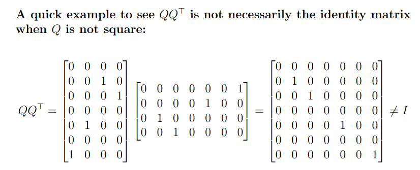
Note that when $Q$ is not square, $Q^{\top }Q=I$ still holds, but $Q{Q}^{\top }=I$ doesn’t necessarily.

Examples:

• 2x2 Rotation matrices are orthogonal
• Permutation matrices are orthogonal

6.3.6 Orthogonal matrices preserve norm and inner product

Orthogonal matrices preserve the norm and inner product of vectors. In other words, if $Q\in {\mathbb{R}}^{n\times n}$ is orthogonal, then, for all $x,y\in {\mathbb{R}}^n$ $||Qx||=||x||\text{ and }(Qx{)}^{\top }(Qy)=x^{\top }y$

Proof: $(Qx{)}^{\top }(Qy)=x^{\top }{Q}^{\top }Qy=x^{\top }Iy=x^{\top }y$. since $Q^{\top }Q=I$. We can use this same argument for the first equality thus $||Qx|{|}^2=(Qx{)}^{\top }(Qx)=x^{\top }x=||x|{|}^2$ and note that $||Qx||\ge 0$ and $||x||\ge 0$ thus it suffices to show that the squares are equal.

6.3.7 Projections with Orthogonal matrices

Let $S$ be a subspace of ${\mathbb{R}}^m$ and $q_1,\dots ,q_n$ be an orthonormal basis for $S$. Let $Q$ be the $m\times n$ matrix whose columns are the $q_i$‘s. Then the projection matrix that projects to $S$ is given by $Q{Q}^{\top }$ and the least squares solution to $Qx=b$ is given by $\hat{x}=Q^{\top }b$.

This is the case because $A^{\top }A$ simplifies to $I$ in the case where our $A$ is orthogonal. Thus $P=A(A^{\top }A{)}^{-1}{A}^{\top }$ simplifies to $P=A{A}^{\top }$.

How to get an Orthonormal Basis: Gram-Schmidt

Algorithm to normalize two vectors: (Gram-Schmidt with 2 only)

1. Normalise $a_1$ to get $q_1=\frac{a_1}{||a_1||}$.
2. Project $a_2$ onto $q_1$ using $pro{j}_{q_1}(a_2)=\frac{q_1{q}_1^{\top }}{q_1^{\top }{q}_1}{a}_2$. Since $q_1$ is normalised (norm 1), we have $pro{j}_{q_1}(a_2)=q_1{q}_q^{\top }{a}_2=(a_2^{\top }{q}_1)q_1$.
3. Subtract the projection of $a_2$ on $q_1$ we just calculated from $a_2$ to get $q_2^{\prime }=a_2-(a_2^{\top }{q}_1)q_1$.
4. Normalise $q_2^{\prime }$ to get $q_2$.

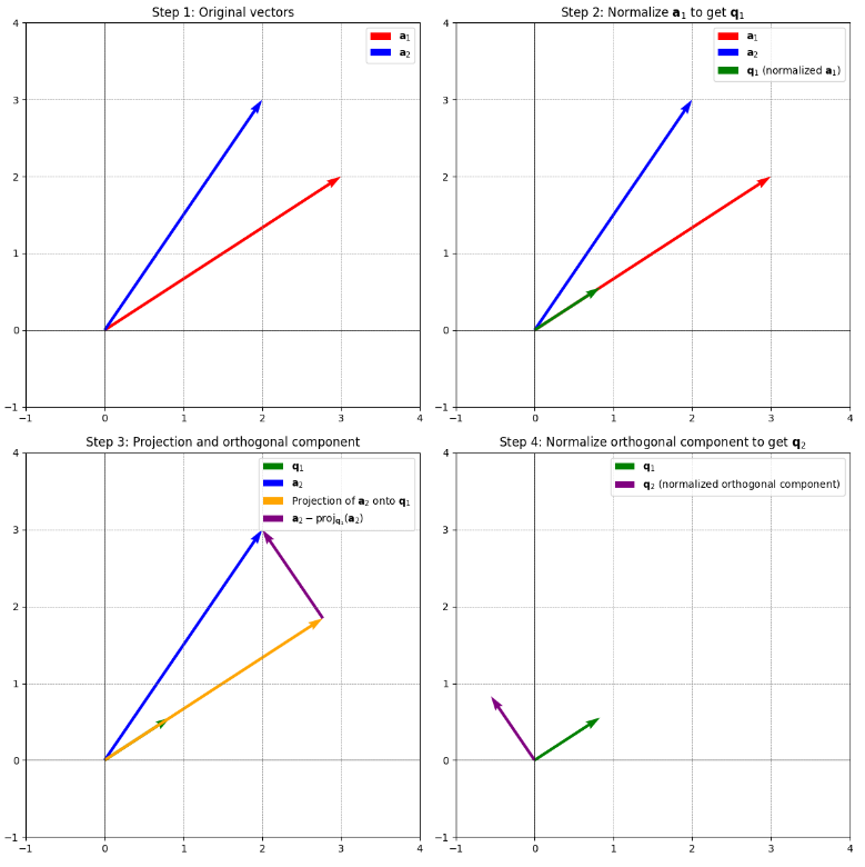
We project $a_2$ onto $q_1$ and then subtract that since we want to remove the part of $a_2$ that is in the direction of $q_1$ to get orthogonal vectors.

Algorithm (Gram-Schmidt):

• $q_1=\frac{a_1}{||a_1||}$
• For $k=2,\dots ,n$ set \begin{align*} q'_k =& a_k - \sum_{i = 1}^{k - 1} (a_k^\top q_i)q_i \\ q_k =& \frac{q_k'}{||q'_k} \end{align*} Linearly dependent case (not in lecture) (i.e. the vectors don’t form a basis) Since in a linearly dependent set of vectors one of them is a linear combination of the previous ones, you’d get $0$ in the subtraction step for it. By excluding those $0$‘s you’d still get an orthonormal basis.

QR-Decomposition

For an $A$ with linearly independent columns, let $Q$ be the result of G-S. Then define $R=Q^{\top }A$. $R$ is upper triangular because each $q_k$ is orthogonal to every $a_i$ for $i<k$ (all after it). Note that $Q$ not necessarily square and thus not invertible.

You can see here, since $q_2,\dots ,q_m$ are by construction orthogonal to $q_1$ thus $a_1$, all entries below $1$ in the first column are $0$. The same goes for all entries below $2$ in the second column.

$Q{Q}^{\top }$ is the projection on the span of the $q_i$‘s and thus also on the $a_i$‘s ($C(Q)=C(A)$). Thus $Q{Q}^{\top }A=A$ and therefore $QR=Q{Q}^{\top }A=A$.

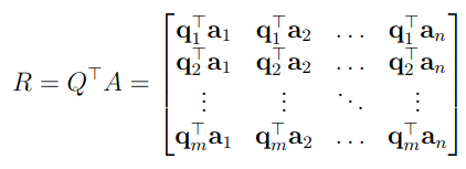
6.3.10 QR-Decomposition

Let $A$ be an $m\times n$ matrix with linearly independent columns. The QR decomposition is given by $A=QR$where

• $Q$ is an $m\times n$ matrix with orthonormal columns (they are the output of Gram-Schmidt)
• $R$ is an upper triangular matrix given by $R=Q^{\top }A$.

6.3.11 R is upper triangular and invertible

The matrix $R$ defined in 6.3.10 is upper triangular and invertible. Moreoever, $Q{Q}^{\top }A=A$ and hence $A=QR$ is well defined.

We have $N(A)=\{0\}$ since $A$ has independent columns and thus $N(R)=\{0\}$. Thus $R\in {\mathbb{R}}^{n\times n}$ (square) must be invertible.

Fact 6.3.12 The QR decomposition greatly simplifies calculations involving Projections and Least Squares:

1. Since $C(A)=C(Q)$ then projetions on $C(A)$ can be done with $Q$: $pro{j}_{C(A)}(b)=Q{Q}^{\top }b$.
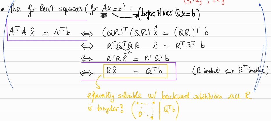
2. The least squares solution to $Ax=b$ denoted $\hat{x}$ is defined as a solution of the normal equations $A^{\top }A\hat{x}=A^{\top }b$Furthermore $A^{\top }A=(QR{)}^{\top }(QR)=R^{\top }{Q}^{\top }QR=R^{\top }R$ and thus $R^{\top }R\hat{x}=R^{\top }{Q}^{\top }b$Since $R$ is invertible we can simplify this to $R\hat{x}=Q^{\top }b$which can efficiently be solved by back substitution since $R$ is a triangular matrix.

6.4 Pseudoinverse

Given $Ax=b$, we can find $x$ by applying $A^{-1}$ if $A$ is invertible: $x=A^{-1}b$. But if $A$ is not invertible, we want to find a matrix $A^{†}$ which accomplishes a similar job as the actual inverse: $A^{†}b$ should give us $x$.

Prelude

$A$ is a linear transformation $A:{\mathbb{R}}^n\to {\mathbb{R}}^m$ with $x\to Ax$. The inverse $A^{†}$ should be a function from $A:{\mathbb{R}}^m\to R^n$ with $Ax\to x$.

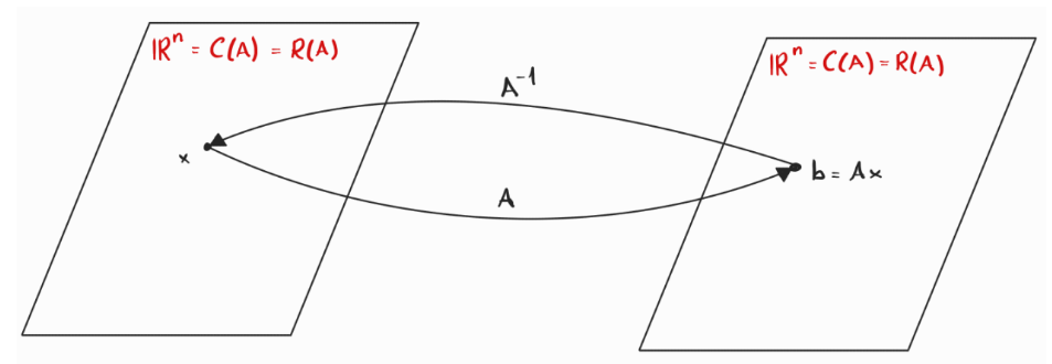
If $A$ is invertible, then $A$ must be square so we have a mapping from ${\mathbb{R}}^n\to {\mathbb{R}}^n$: This $A$ is bijective, it perfectly reverses.

If $A\in {\mathbb{R}}^{m\times n}$ with independent columns (full column-rank), we can visualise $A$ as suc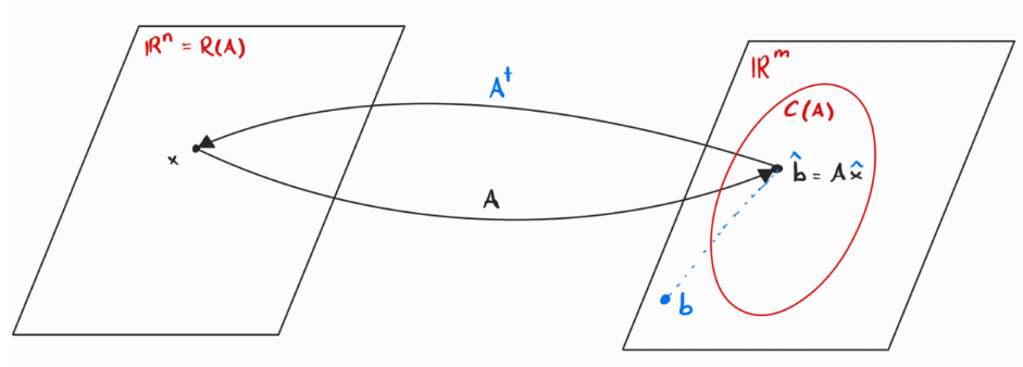h: The column space $C(A)$ is just part of the whole ${\mathbb{R}}^m$. We first have to project $b$ into $C(A)$ $pro{j}_{C(A)}(b)=\hat{b}$, before we can invert it. By inverting, we map $\hat{b}$ back to $\hat{x}$, i.e. we find an $\hat{x}$ that brings us closest to $b$, which is exactly Least Squares.

If $A\in {\mathbb{R}}^{m\times n}$ with independent rows (full row-rank), we can visualise $A$ as suc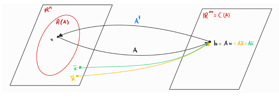h: There are multiple $x\in {\mathbb{R}}^n$ that map to $b$ via $Ax$, and we have to find one to which we invert. We pick one with the smallest norm $||x|{|}^2$ minimal. By Lemma 6.4.5 we know that the smallest such $x$ is an $x\in R(A)=C(A^{\top })$. Since $A$ does not have full column rank, $A$ has a non-trivial nullspace, and thus the solution space of $Ax=b$ is $x_r+x_n$. If we take the unique vector in $C(A^{\top })$, we basically set $x_n$ to $0$, thus making sure the norm is minimal.

If $A$ has neither full column nor full row-rank, we have to solve both problems at once. We then decompose $A=CR$ (with $C$ full column-rank and $R$ full row-rank). Then $A^{†}=R^{†}{C}^{†}$.

6.4.1 Definitions

6.4.1 Pseudoinverse for matrices of full column rank

For $A\in {\mathbb{R}}^{m\times n}$ with $\text{rank}(A)=n$, we define the pseudo-inverse $A^{†}\in {\mathbb{R}}^{n\times m}$ as $A^{†}=(A^{\top }A{)}^{-1}{A}^{\top }$

6.4.2 Left Inverse

For $A\in {\mathbb{R}}^{m\times n}$ with $\text{rank}(A)=n$, the pseudoinverse $A^{†}$ is a left inverse of $A$, meaning $A^{†}A=I$

Proof: Since $A$ has full column rank, $A^{\top }A$ invertible and then $A^{†}A=((A^{\top }A{)}^{-1}{A}^{\top })A$ $=(A^{\top }A{)}^{-1}(A^{\top }A)=I$.

6.4.3 Pseudoinverse for matrices with full row rank

For $A\in {\mathbb{R}}^{m\times n}$ with $\text{rank}(A)=m$, we define the pseudo-inverse $A^{†}\in {\mathbb{R}}^{n\times m}$ as $A^{†}=A^{\top }(A{A}^{\top }{)}^{-1}$

For an $A$ with full column-rank, we basically define, $A^{†}$ as the transpose of the pseudoinverse of the transpose: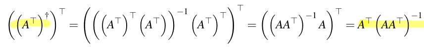

6.4.4 Right inverse

For $A\in {\mathbb{R}}^{m\times n}$ with $\text{rank}(A)=m$, the pseudo-inverse $A^{†}\in {\mathbb{R}}^{n\times m}$ is a right inverse of $A$: $A{A}^{†}=I$

Proof Since $A^{\top }$ has full column rank, $((A^{\top }{)}^{\top }{A}^{\top })=A{A}^{\top }$ is invertible: $A{A}^{†}=A{A}^{\top }(A{A}^{\top }{)}^{-1}=I$.

Since for $A$ full row rank there are many possible solutions, the pseudoinverse is choosing the one with the smallest norm $||x|{|}^2$ such that $Ax=b$. Since each solution is $x=x_r+x_n$ with $x_r\in R(A)=C(A^{\top })$ and $x_n\in N(A)$, the pseudoinverse chooses an $x=x_r+0$ with no nullspace component to get the smallest norm. Notice the $A^{\top }$ at the front of the definition. This means that $\hat{x}$ is in the row-space: exactly what we want!

6.4.5 & 6.4.6 Unique Solution for full row rank

For any matrix $A$ and a vector $b\in C(A)$, the unique solution to ${\min }_{x\in {\mathbb{R}}^n}||x|{|}^2\text{ s.t. }Ax=b$ is given by the vector $\hat{x}\in C(A^{\top })$ that satisfies $A\hat{x}=b$.

For a full row rank matrix $A$, the unique solution is given by the vector $\hat{x}=A^{†}b$.

Proof By Lemma 6.4.5 we only need to show that $\hat{x}=A^{†}b$ satisfies $A\hat{x}=b$ and that $\hat{x}\in C(A^{\top })$.

• $A\hat{x}=A{A}^{†}b=A{A}^{\top }(A{A}^{\top }{)}^{-1}b=b$
• $\hat{x}=A^{†}b=A^{\top }((A{A}^{\top }{)}^{-1}b)=A^{\top }y$ for some $y$ thus $x\in C(A^{\top })$

6.4.7 Pseudoinverse for all matrices

For $A\in {\mathbb{R}}^{m\times n}$ with $\text{rank}(A)=r$ and CR decomposition $A=CR$, we define the pseudoinverse $A^{†}$ as $A^{†}=R^{†}{C}^{†}$

We can rewrite this as $A^{†}=R^{\top }{(R{R}^{\top })}^{-1}{(C^{\top }C)}^{-1}{C}^{\top }=$ $R^{\top }{(C^{\top }CR{R}^{\top })}^{-1}{C}^{\top }=$ $R^{\top }{(C^{\top }A{R}^{\top })}^{-1}{C}^{\top }$.

6.4.8 For any $A$

Given $A\in {\mathbb{R}}^{m\times n}$ and a vector $b\in {\mathbb{R}}^m$, the unique solution to ${\min }_{x\in {\mathbb{R}}^n}||x|{|}^2$ such that $A^{\top }Ax=A^{\top }b$ is given by $\hat{x}=A^{†}b$.

6.4.9 Full Rank Factorisation

For $A\in {\mathbb{R}}^{m\times n}$ with $\text{rank}(A)=r$, let $S\in {\mathbb{R}}^{m\times r}$ and $T\in {\mathbb{R}}^{r\times n}$ such that $A=ST$. Then $A^{†}=T^{†}{S}^{†}$

6.4.10 Pseudoinverse Conditions

$A^{†}$ is a pseudoinverse if it satisfies the following conditions:

• $A{A}^{†}A=A$
• $A^{†}A{A}^{†}=A^{†}$
• $(A^{\top }{)}^{†}=(A^{†}{)}^{\top }$
• $A{A}^{†}$ is symmetric (i.e. $(A{A}^{†}{)}^{\top })=A{A}^{†}$). It is the projection matrix on $C(A)$.
• $A^{†}A$ is symmetric (i.e. $(A{A}^{†}{)}^{\top }=A{A}^{†}$). It is the projection matrix on $C(A^{\top })$.

Nullspace of $A^{†}$ and $A^{\top }$: We have $N(A^{\top })=N(A^{†})$. Intuitively this holds as $A^{†}\hat{x}\in C(A^{\top })$ (we pick the minimal $\hat{x}$). Thus anything orthogonal to the subspace $C(A{)}^{\perp }=N(A^{\top })$ is projected to $0$: $\forall x\in C(A{)}^{\perp }$ we have $A^{†}x=0$. We conclude that $N(A^{\top })=C(A{)}^{\perp }=N(A^{†})$.