3. Architecture

3.1 Caches

There are different levels of caching, each of which has different memory speeds.

3.2 Compute Optimisation

We can use:.

• superscalar execution: multiple instructions per cycle
  • this is within a single core (the ALU must support superscalar execution)
  • the pipeline then fetches multiple at the same time, executes at the same time, etc…
• out-of-order execution: reorder instructions to keep the cpu busy

3.2.1 Vectorisation

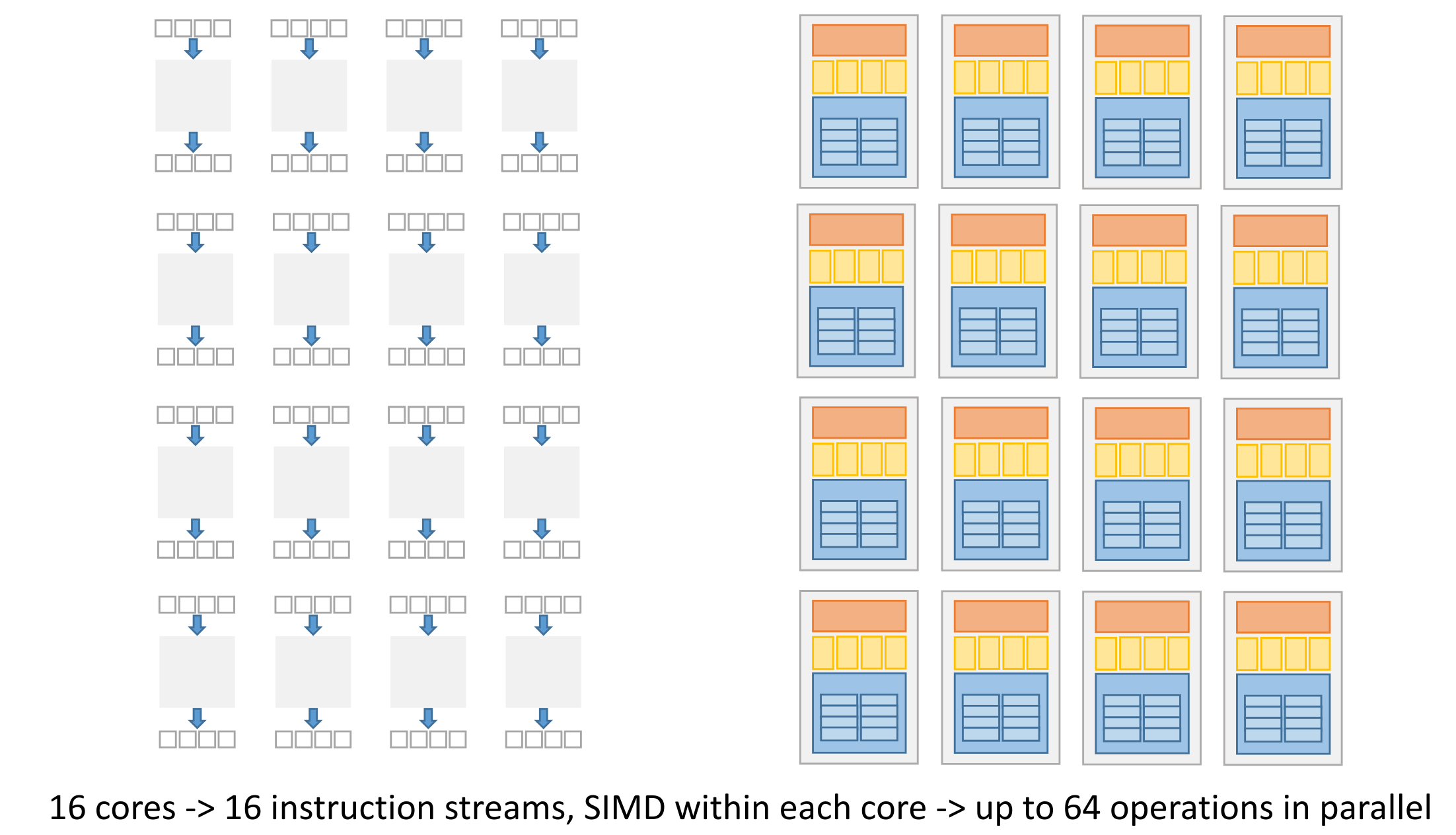
We can use SIMD instructions to parallelise execution of for-loops that apply “mappings” to a long data vector.

3.2.2 Instruction Level Parallelism

1. Dependency analysis:
   1. parallel execution of independent instructions (uses superscalar execution to execute multiple at the same time)
   2. to optimise instruction ordering - keeps the CPU busy. May happen at both compile-time and by the CPU.
2. speculative execution - the CPU can execute a branch before the check finishes in order to keep the CPU busy.

ILP is what happends on a single thread - there’s no concurrency here (single non-interleaved task).
This is hardware dependent, if there’s no support for ILP it’s not possible.

3.2.3 Pipelining

Executing an instruction inside the CPU happens in stages: instruction fetching, decoding, etc…

The time this pipeline takes can be optimised, by balancing it.

Balanced

All stages take the same amount of time.

Previous def. of balanced

Balanced if:

• latency is constant for all elements (no gaps)
• no stage is longer than the first stage

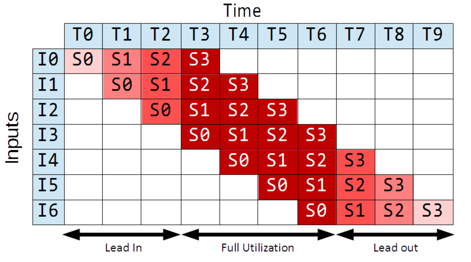
Lead-in and Lead-out

Lead-in (the warm-up phase) and lead-out (cool-down phase) diminish our speedup because they are phases during which the pipeline is not fully saturated.
They diminish our performance gains for short pipelines.

In the above example, due to lead-in and out, we only have throughput of $0.7$ for this finite pipeline, while in infinite time this would be $1$.

Throughput

Amount of work that can be done by a system in a given period of time.
In CPU, number of instructions per second.

(if we have one execution unit per stage) Bound = 1 / max(computation_time(stage) for all stages)

Throughput (finite time)

If we know how many elements need to be processed, we consider lead-in/lead-out time. Number of instances $N$
throughput (with lead-in and -out) = N / (overall time for N elements)
As this goes to infinity (limit), it approaches the result from before.

Throughput is how many, latency is how long.

Latency

Time needed to perform a given computation (e.g. a CPU instruction).
In CPU, time to execute a single instruction.
Latency bound = # stages * max(computation_time(stage) for all stages) THIS IS ONLY FOR A CPU, with a clock ticking!!

The pipeline latency is constant over time, if the pipeline is balanced. Otherwise, it will grow.

Note, the latency usually means the latency of the first instance. But we need to specify if we mean latency of one instance or all stages (sum of all instances).

Note also latency must not constant, if the pipeline is not balanced for example. If the pipeline is not balanced, the latency cannot be bounded.

Latency Calculations

Generally, you can take the total time of the first instance:

$$\text{latency}=\text{total\_time}(\text{first\_instance})=\text{sum}(\text{time}(\text{all\_stages}))$$

If the latency is not constant, we can calculate it for the $n$-th instance:

$$\text{latency}=\text{total\_time}(\text{first\_instance})+(\text{max}({\text{time}}_{\text{stage}})-\text{time\_of\_first\_stage})\cdot (n-1)$$

Bandwidth

The bandwidth is the amount of work done in parallel.

This pipeline is not balanced, the drying step takes double the time of the others. Thus the latency grows as we have more and more loads going through.

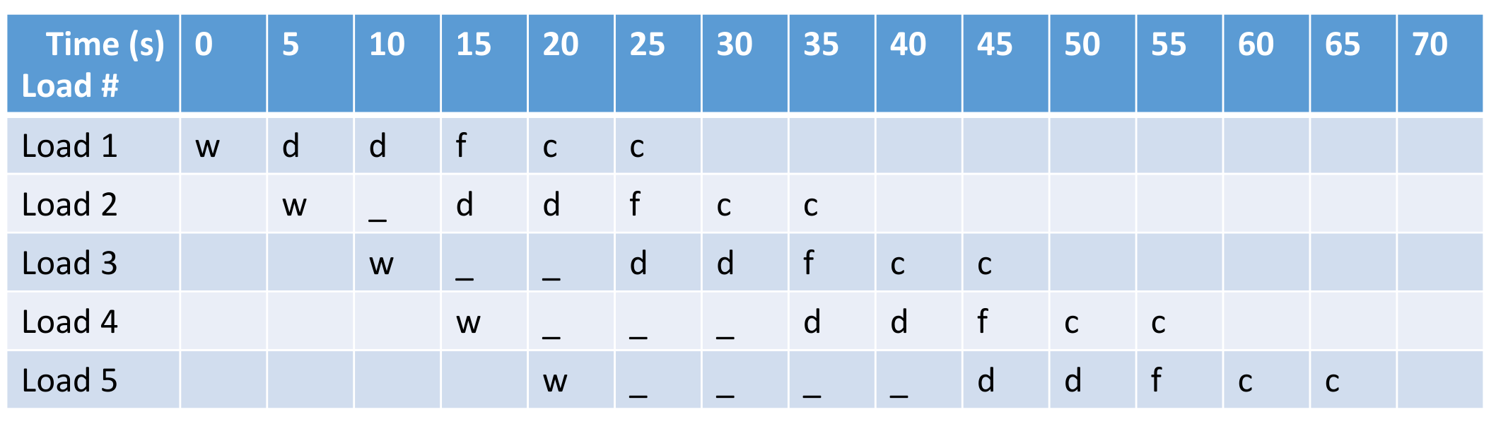
We can split the drying stage into two, in order to fix the latency. However, too much splitting is not practical, as this will lead to enormous overhead when switching.