2. Wahrscheinlichkeitstheorie

2.0 Intro

A fundamental problem in combinatorics is determining the number of ways to choose k items from a set containing n distinct items. The method for counting depends on two crucial questions:

Does the order of selection matter? (Is the selection ordered or unordered?)
Can items be selected more than once? (Is the selection with replacement or without replacement?)

Selection Type	Replacement?	Order Matters?	Formula
Tuple	Yes	Yes	$n^{k}$
k-Permutation	No	Yes	$n^{\underline{k}} = \frac{n !}{( n - k )!}$
Combination / Set	No	No	$(k n) = \frac{n !}{k ! ( n - k )!}$
Multiset / Stars and Bars	Yes	No	$(k n + k - 1) = (n - 1 n + k - 1)$

2.0.1 Ordered Selection with Replacement - Tuples

Derivation: This uses the basic multiplication principle of counting. We have $k$ independent choices to make, and each choice has $n$ possibilities.

Total ways = (Choices for slot 1) $\times$ (Choices for slot 2) $\times \dots \times$ (Choices for slot k)
Total ways = $n \times n \times \dots \times n$ ( $k$ times)

Formula: The number of ways is $n^{k}$ . We get an ordered list of length $k$ , often called a tuple.

Possible 4-digit PIN codes using digits 0-9 ( $n = 10, k = 4$ ): $1 0^{4} = 10000$ .
Possible outcomes when rolling a die 3 times ( $n = 6, k = 3$ ): $6^{3} = 216$ . (e.g., (1, 6, 1) is different from (6, 1, 1)).

2.0.2 Ordered Selection without Replacement - k-Permutations

Think of filling $k$ ordered slots.

For the first slot, we have $n$ choices.
Since we cannot replace the chosen item, we only have $n - 1$ choices remaining for the second slot.
For the third slot, we have $n - 2$ choices, and so on, until the $k$ -th slot, for which we have $n - (k - 1) = n - k + 1$ choices.

Derivation: Using the multiplication principle with decreasing choices:

Total ways = (Choices for slot 1) $\times$ (Choices for slot 2) $\times \dots \times$ (Choices for slot k)
Total ways = $n \times (n - 1) \times (n - 2) \times \dots \times (n - k + 1)$

Formula: This quantity is often denoted as $n^{\underline{k}}$ (falling factorial) or $P (n, k)$ . It can also be expressed using factorials:

$n^{\underline{k}} = \frac{n !}{( n - k )!}$
Recall that $n! = n \times (n - 1) \times \dots \times 2 \times 1$ .

Result Type: An ordered list of $k$ distinct items, often called a k-permutation of $n$ .

Ways to award Gold, Silver, Bronze medals in a race with 8 competitors ( $n = 8, k = 3$ ): $8^{\underline{3}} = 8 \times 7 \times 6 = 336$ .
Ways to arrange 3 distinct books from a collection of 5 on a shelf ( $n = 5, k = 3$ ): $5^{\underline{3}} = 5 \times 4 \times 3 = 60$ .

2.0.3 Unordered Selection without Replacement - Combinations / Sets

Intuition: How is this related to the ordered case without replacement (Case 2)? In Case 2, we counted sequences like (A, B, C) and (C, B, A) as distinct outcomes. However, if the order doesn’t matter, these sequences correspond to the same selection: the set ${A, B, C}$ . We need to figure out how many ordered sequences correspond to each unordered set.

Derivation:

Start with the ordered count: $n^{\underline{k}} = \frac{n !}{( n - k )!}$ ordered ways to select $k$ distinct items.
Identify overcounting: There are $k!$ ways to order $k$ distinct items (k choices for the first position, k-1 for the second, etc.).
Correct for overcounting: Divide the ordered count by the overcounting factor $k!$

Formula: Number of unordered sets = $\frac{Number of ordered sequences}{Number of ways to order each set} = \frac{n ^{\underline{k}}}{k !}$
This is the binomial coefficient, read as “n choose k”:

$(k n) = \frac{n ^{\underline{k}}}{k !} = \frac{n !}{k ! ( n - k )!}$

Symmetry of Combinations

Note that $(k n) = (n - k n)$ .
Choosing $k$ items to include is the same as choosing $n - k$ items to exclude.

Result Type: An unordered set of $k$ distinct items, often called a combination.
Examples:

Ways to choose 3 winners from 10 lottery tickets (order doesn’t matter) ( $n = 10, k = 3$ ): $(3 10) = \frac{10 \times 9 \times 8}{3 \times 2 \times 1} = 120$ .
Ways to form a 5-card poker hand from a 52-card deck ( $n = 52, k = 5$ ): $(5 52) = \frac{52 !}{5 ! 47 !} = 2, 598, 960$ .

4. Unordered Selection with Replacement - Multisets / Stars and Bars

Intuition: $n$ bins, representing the $n$ distinct types of items we can choose from. Choose a total of $k$ items.
Since order doesn’t matter and we can repeat types, this is like deciding how many times we choose type 1, how many times type 2, …, up to type $n$ , such that the total number of choices is $k$ .

Derivation (Stars and Bars technique):

Represent Choices: Let $k$ “stars” $(*)$ represent the $k$ items we need to choose. Our goal is to divide these stars into $n$ groups, where each group corresponds to one of the $n$ types of items.
Represent Dividers: To divide the stars into $n$ groups, we need $n - 1$ “bars” (|). For example, if we have $n = 4$ types and want to choose $k = 5$ items, the sequence **|*||** could represent choosing 2 items of type 1, 1 item of type 2, 0 items of type 3, and 2 items of type 4.
Combine Stars and Bars: Every possible selection corresponds uniquely to an arrangement of $k$ stars and $n - 1$ bars in a sequence.
Counting Arrangements: We have a total of $k + (n - 1)$ positions in the sequence. We need to determine where the $k$ stars (or equivalently, the $n - 1$ bars) go.
Apply Combination Formula: This is now a combination problem (Case 3)! We need to choose $k$ positions for the stars out of the $k + n - 1$ total positions. The number of ways to do this is $(k k + n - 1)$ . Alternatively, we could choose $n - 1$ positions for the bars out of the $k + n - 1$ total positions, which gives $(n - 1 k + n - 1)$ . These two binomial coefficients are equal.

Formula: $(k n + k - 1) = (n - 1 n + k - 1)$ We get an unordered collection where repetitions are allowed, often called a multiset.

Examples:

Ways to choose 3 scoops of ice cream from 5 available flavours ( $n = 5, k = 3$ ): $(3 5 + 3 - 1) = (3 7) = \frac{7 \times 6 \times 5}{3 \times 2 \times 1} = 35$ .
Number of non-negative integer solutions to $x_{1} + x_{2} + x_{3} = 10$ ( $n = 3$ types/variables, $k = 10$ total value/items): $(10 3 + 10 - 1) = (10 12) = (2 12) = \frac{12 \times 11}{2} = 66$ .

2.1 Grundbegriffe & Notationen

2.1 Diskreter Wahrscheinlichkeitsraum

Ein diskreter Wahrscheinlichkeitsraum ist bestimmt durch eine Ergebnismenge $Ω = {ω_{1}, ω_{2}, ...}$ von Elementarereignissen.
Jedem Elementarereignis $ω_{i}$ ist eine (Elementar-)Wahrscheinlichkeit $Pr [ω_{i}]$ zugeordnet, wobei wir fordern, dass $0 \leq Pr [ω_{i}] \leq 1$ und
$ω \in Ω \sum Pr [ω] = 1$

$Ω$ kann endlich oder unendlich (sogar überabzählbar unendlich) sein.

Ereignis

Eine Menge $E \subseteq Ω$ heisst Ereignis. Die Wahrscheinlichkeit $P r [E]$ eines Ereignisses ist definiert durch
$Pr [E] := ω \in E \sum Pr [ω]$

Komplementärereignis

Ist $E$ ein Ereignis, so bezeichnen wir mit $\overline{E} := Ω ∖ E$ das Komplementärereignis.

Properties of Sets and Complements:
All Standard rules (Assoc., Identity, Distrib.) apply.

$(A^{C} \cap B^{C} \cap C^{C}) = (A \cup B \cup C)^{C}$ (De Morgan)

$A \cup Ω = Ω$ and $A \cap \emptyset = \emptyset$
$A \cup A^{c} = Ω$ and $A \cap A^{c} = \emptyset$ and $(A^{c})^{c} = A$
$A \cup (A \cap B) = A$ and $A \cap (A \cup B) = A$

Disjointification (useful for probability)

$A \cup B = A ⊔ (B \cap A^{c})$ : turns a union into a disjoint union
$B = (B \cap A) ⊔ (B \cap A^{c})$ : partition $B$ by $A$
More generally, if ${A_{i}}$ partitions $Ω$ : $B = ⨆_{i} (B \cap A_{i})$

2.2 Funamental Properties

$Pr [\emptyset] = 0$ , $Pr [Ω] = 1$

$0 \leq Pr [A] \leq 1$

$Pr [\overline{A}] = 1 - Pr [A]$

Wenn $A \subseteq B$ so folgt $Pr [A] \leq Pr [B]$

Für paarweise disjunkte Ereignisse gilt der folgende Satz.

2.3 Additionssatz

Wenn für die Ereignisse $A_{1}, \dots, A_{n}$ paarweise disjunkt sind, so gilt
$Pr [i = 1 ⋃ n A_{i}] = i = 1 \sum n Pr [A_{i}]$

Im allgemeinen Fall können wir mit der Siebformel arbeiten.

2.5 Siebformel

Für Ereignisse $A_{1}, \dots, A_{n}$ ( $n \geq 2$ ) gilt
$Pr [i = 1 ⋃ n A_{i}] = l = 1 \sum n (- 1)^{l + 1} 1 \leq i_{1} \leq \dots \leq i_{l} \leq n \sum P r [A_{i_{1}} \cap \dots \cap A_{i_{l}}]$

Der Union-Bound (Boolsche Ungleichung) wird öfters genutzt, da er einfacher anzuwenden ist. Er folgt direkt aus der Siebformel.

Boolsche Ungleichung

Für Ereignisse $A_{1}, \dots, A_{n}$ gilt
$Pr [i = 1 ⋃ n A_{i}] \leq i = 1 \sum n Pr [A_{i}]$

Beweis:

Sei $B_{i} := A_{i} ∖ (A_{1} \cup \dots \cup A_{i - 1})$
Dann gilt $Pr [B_{i}] \leq Pr [A_{i}]$ (weil $B_{i} \subseteq A_{i}$ )
Alle $B_{i}, B_{j}$ sind disjunkt und $⋃_{i = 1}^{n} A_{i} = ⋃_{i = 1}^{n} B_{i}$
Per Additionssatz (weil alle $B_{i}$ disjunkt) gilt

Pr [i = 1 ⋃ n A_{i}] = Pr [i = 1 ⋃ n B_{i}] = \sum Pr [B_{i}] \leq i = 1 \sum n Pr [A_{i}]

Laplace Raum

In einem Laplace-Raum sind alle Elementarereignisse gleich wahrscheinlich. Deswegen gilt $Pr [E] = \frac{∣ E ∣}{∣Ω∣}$ .

$Ω$ wird dann uniform verteilt genannt.

Man sagt auch, dass $Pr [ω] = 1/∣Ω∣$ für alle $ω$ die größtmögliche Entropie hat.

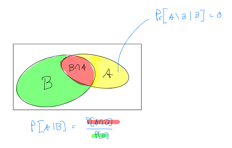
2.2 Bedingte Wahrscheinlichkeiten

Durch das Bekanntwerden zusätzlicher Information verändern sich Wahrscheinlichkeiten.

Wir notieren $Pr [A ∣ B]$ die Wahrscheinlichkeit von $A$ , wenn wir wissen, dass $B$ eingetreten ist.

Es gilt dann:

$Pr [B ∣ B] = 1$ und $Pr [B ∣ \overline{B}]$
$Pr [A ∣ Ω] = Pr [A]$ da ” $Ω$ ist eingetreten” keine extra Information liefert.
Wenn $B$ eingetreten ist, kann nur noch $Pr [A \cap B]$ eintreten. Daher ist $Pr [A ∣ B]$ proportional zu $Pr [A \cap B]$

2.8 Bedingte Wahrscheinlichkeit

$A$ und $B$ seien Ereignisse mit $Pr [B] > 0$ . Die bedingte Wahrscheinlichkeit $Pr [A ∣ B]$ von $A$ gegeben $B$ ist definiert durch
$Pr [A ∣ B] := \frac{Pr [ A \cap B ]}{Pr [ B ]}$

Die bedingten Wahrscheinlichkeiten $Pr [\circ ∣ B]$ bilden einen neuen Wahrscheinlichkeitsraum. Es gilt $\sum_{ω \in Ω} Pr [ω ∣ B]$ $= \sum_{ω \in Ω} \frac{P r [ ω \cap B ]}{P r [ B ]} = \sum_{ω \in B} \frac{P r [ ω ]}{P r [ B ]}$ $= \frac{P r [ B ]}{P r [ B ]} = 1$ .
Damit gelten alle Rechenregeln auch für bedingte Wahrscheinlichkeiten, z.B.

$Pr [\emptyset∣ B] = 0$
$Pr [\overline{A} ∣ B] = 1 - Pr [A ∣ B]$

Die Wahrscheinlichkeiten für alle Ereignisse $ω \in \overline{B}$ (außerhalb $B$ ) werden auf $0$ gesetzt. Der Rest wird dann skaliert, damit die Summe wieder $1$ ergibt (mit $1/ Pr [B]$ , welcher in der Formel auftaucht).

2.10 Multiplikationssatz

Seien die Ereignisse $A_{1}, \dots, A_{n}$ gegeben. Falls $Pr [A_{1} \cap \dots \cap A_{n}] > 0$ ist, gilt
$Pr [A_{1} \cap \dots \cap A_{n}] = Pr [A_{1}] \cdot Pr [A_{2} ∣ A_{1}] \cdot Pr [A_{3} ∣ A_{1} \cap A_{2}] \dots Pr [A_{n} ∣ A_{1} \cap \dots \cap A_{n - 1}]$

Beweis

Da $Pr [A_{1}] \geq Pr [A_{1} \cap A_{2}] \geq \dots \geq Pr [A_{1} \cap \dots \cap A_{n}] > 0$ sind alle W’keiten wohldefiniert
Wir schreiben um zu

\frac{Pr [ A _{1} ]}{1} \cdot \frac{Pr [ A _{1} \cap A _{2} ]}{Pr [ A _{1} ]} \cdot \frac{Pr [ A _{1} \cap A _{2} \cap A _{3} ]}{Pr [ A _{1} \cap A _{2} ]} \dots \frac{Pr [ A _{1} \cap \dots \cap A _{n} ]}{Pr [ A _{1} \cap \dots \cap A _{N - 1} ]}

man sieht leicht dass sich hier kreuzweise alles bis auf $Pr [A_{1} \cap \dots \cap A_{n}]$ herauskürzt.

2.13 Satz von der totalen W'keit

Die Ereignisse $A_{1}, \dots, A_{n}$ seien paarweise disjunkt und es gelte $B \subseteq A_{1} \cup \dots \cup A_{n}$ . Dann folgt
$Pr [B] = i = 1 \sum n Pr [B ∣ A_{i}] \cdot Pr [A_{i}]$

Proof

$B = (B \cap A_{1}) \cup \dots \cup (B \cap A_{n})$ da $B \subseteq A ....$ ist.
Da alle $A_{X}$ disjunkt sind, sind auch $B \cap A_{i}$ und $B \cap A_{j}$ disjunkt.
Dann gilt $Pr [B \cap A_{i}] = Pr [B ∣ A_{i}] \cdot Pr [A_{i}]$
Wir wenden den Additionssatz an

Pr [B] = Pr [B \cap A_{1}] + \dots + Pr [B \cap A_{n}] = Pr [B ∣ A_{1}] \cdot Pr [A_{1}] + \dots + Pr [B ∣ A_{n}] \cdot Pr [A_{n}]

2.15 Satz von Bayes

Die Ereignisse $A_{1}, \dots, A_{n}$ seien paarweise disjunkt. Ferner sei $B \subseteq A_{1} \cup \dots \cup A_{n}$ ein Ereignis $Pr [B] > 0$ .
Dann gilt für ein beliebiges $i = 1, \dots, n$ :
$Pr [A_{i} ∣ B] = \frac{Pr [ A _{i} \cap B ]}{Pr [ B ]} = \frac{Pr [ B ∣ A _{i} ] \cdot Pr [ A _{i} ]}{\sum _{j = 1}^{n} Pr [ B ∣ A _{j} ] \cdot Pr [ A _{j} ]}$

Wir können mit dem Satz von Bayes gewissermaßen die Reihenfolge der Bedingung umdrehen.

2.3 Unabhängigkeit

2.18 Unabhängigkeit (2 Ereignisse)

Die Ereignisse $A$ und $B$ heißen unabhängig, wenn gilt
$Pr [A \cap B] = Pr [A] \cdot Pr [B]$

Wenn $Pr [B] \neq = 0$ so können wir Umformen zu $Pr [A] = \frac{P r [ A \cap B ]}{P r [ B ]} = Pr [A ∣ B]$ .

Intuitiv, wenn wir wissen, dass $A$ eingetreten ist so ändert sich nichts an der Wahrscheinlichkeit mit der wir $C$ erwarten.

Für mehr als 2 Ereignisse wird die Definition etwas komplexer:

Beispiel: Wir werfen zwei ideale Münzen $M_{1}$ und $M_{2}$ : $Ω := {(K, K), (K, Z), (Z, K), (Z, Z)}$ , $Pr [A] = 1/4$ .

A B C := " M_{1} zeigt Kopf" = {(K, K), (K, Z)} := " M_{2} zeigt Kopf" = {(K, K), (Z, K)} := "die Resultate sind verschieden" = {(K, Z), (Z, K)} .

$A$ und $B$ voneinander unabhängig, denn $Pr [A \cap B] = 1/4 = Pr [A] Pr [B] .$
$B$ und $C$ voneinander unabhängig
genauso $A$ und $C$
Allerdings sind $A$ , $B$ , und $C$ zusammen nicht voneinander unabhängig, denn falls je zwei Ereignisse eintreten, so tritt auf keinen Fall das Dritte ein, also insbesondere $Pr [A \cap B \cap C] = 0 \neq = 1/8 = Pr [A] Pr [B] Pr [C]$ .
Die paarweise Unabhängigkeit der Ereignisse genügt nicht → $Pr [A_{1} \cap \dots \cap A_{n}] = Pr [A_{1}] \dots Pr [A_{n}]$ muss auch gelten

Beispiel: Wir wählen eine zufällige Zahl zwischen 1 und 8 und betrachten die Ereignisse $A := "die Zahl ist in {1, 2, 3, 4} "$ und $B := "die Zahl ist in {1, 5, 6, 7} "$ . Außerdem sei $C = B$ .

Pr [A \cap B \cap C] = Pr [A \cap B] = 1/8 = Pr [A] Pr [B] Pr [C],

- Aber $\Pr[A \cap B] = 1/8 \neq \Pr[A]\Pr[B]$, das heißt, $A$ und $B$ sind nicht unabhängig.

Wir brauchen also beide Bedingungen gleichzeitig.

Definition 2.22 (Unabhängigkeit von $n$ Ereignissen)

Die Ereignisse $A_{1}, \dots, A_{n}$ heissen unabhängig, wenn für alle Teilmengen $I \subseteq {1, \dots, n}$ mit $I = {i_{1}, \dots, i_{k}}$ gilt, dass
$Pr [A_{i_{1}} \cap \dots \cap A_{i_{k}}] = Pr [A_{i_{1}}] \dots Pr [A_{i_{k}}]$

Eine unendliche Familie von Ereignissen $A_{i}$ mit $i \in N$ heißt unabhängig, wenn dies für jede endliche Teilmenge $I \subseteq N$ erfüllt ist.

Lemma 2.23

Die Ereignisse $A_{1}, \dots, A_{n}$ sind genau dann unabhängig, wenn für alle $(s_{1}, \dots, s_{n}) \in {0, 1}^{n}$ gilt, dass
$Pr [A_{1}^{s_{1}} \cap \dots \cap A_{n}^{s_{n}}] = Pr [A_{1}^{s_{1}}] \dots Pr [A_{n}^{s_{n}}]$
wobei $A_{i}^{0} = \overset{ˉ}{A}_{i}$ und $A_{i}^{1} = A_{i}$ .

Beobachtung: Aus Lemma 2.23 folgt, dass für $A$ und $B$ unabhängig auch $\overline{A}$ , $B$ oder $A$ , $\overline{B}$ und $\overline{A}$ , $\overline{B}$ unabhängig sind.

Lemma 2.24

Seien $A$ , $B$ und $C$ unabhängige Ereignisse. Dann sind auch $A \cap B$ und $C$ bzw. $A \cup B$ und $C$ unabhängig.

Beweis: Die Unabhängigkeit von $A \cap B$ und $C$ folgt aus $Pr [(A \cap B) \cap C] = Pr [A] Pr [B] Pr [C] = Pr [A \cap B] Pr [C]$ . Mit der Inklusion-Exklusion-Formel gilt:

Pr [(A \cup B) \cap C] = Pr [(A \cap C) \cup (B \cap C)] = Pr [A \cap C] + Pr [B \cap C] - Pr [A \cap B \cap C] = Pr [C] \cdot (Pr [A] + Pr [B] - Pr [A \cap B]) = Pr [A \cup B] \cdot Pr [C],

und daraus folgt die Unabhängigkeit von $A \cup B$ und $C$ .

2.4 Zufallsvariablen

Definition 2.25 (Zufallsvariable)

Eine Zufallsvariable ist ein Abbildung $X : Ω \to R$ , wobei $Ω$ die Ergebnismenge eines Wahrscheinlichkeitsraumes ist.

Wertebereich einer Zufallsvariable

Bei diskreten Wahrscheinlichkeitsräumen ist der Wertebereich einer Zufallsvariablen
$W_{X} := X (Ω) = {x \in R ∣ \exists ω \in Ω mit X (ω) = x}$

Sei $W_{X} = {x_{1}, \dots, x_{n}}$ bzw. $W_{X} = {x_{1}, x_{2}, \dots}$
Für ein beliebiges $1 \leq i \leq n$ sei das Ereignis $X^{- 1} (x_{i}) = {ω \in Ω ∣ X (ω) = x_{i}}$ (wir drehen hier quasi um).
Beachte, $X^{- 1} (x_{i})$ schreibt man häufig als $" X = x_{i} "$ .

Pr [" X \leq x_{i} "] = x \in W_{X} : x \leq x_{i} \sum Pr [" X = x "] = Pr [{ω \in Ω ∣ X (ω) \leq x_{i}}] .

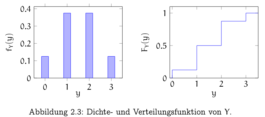
Dichefunktion

Die Funktion
$f_{X} : R \to [0, 1], x \mapsto Pr [X = x]$
nennt man Dichte(funktion) von $X$ .

Verteilungsfunktion

Die Funktion
$F_{X} : R \to [0, 1], x \mapsto Pr [X \leq x] = x^{'} \in W_{X} : x^{'} \leq x \sum Pr [X = x^{'}]$
heisst Verteilung(sfunktion) von $X$ .

Beachte, Dichte/Verteilungsfunktion beschreiben eine Zufallsvariable eindeutig.

2.4.1 Erwartungswert

Definition 2.27 (Erwartungswert)

Zu einer Zufallsvariablen $X$ definieren wir den Erwartungswert $E [X]$ durch
$E [X] := x \in W_{X} \sum x \cdot Pr [X = x]$

Beachte, bei unendlichen Wahrscheinlichkeitsräumen kann diese Serie divergieren. Dann sagen wir, dass der Erwartungswert undefiniert ist.

Beispiel: Der Erwartungswert $E [Y]$ für die Anzahl “Kopf” bei dreimaligen Werfen einer idealen Münze ist

E [Y] = i = 0 \sum 3 i \cdot Pr [Y = i] = 1 \cdot Pr [Y = 1] + 2 \cdot Pr [Y = 2] + 3 \cdot Pr [Y = 3] = 1 \cdot \frac{3}{8} + 2 \cdot \frac{3}{8} + 3 \cdot \frac{1}{8} = \frac{3}{2},

Lemma 2.29

Ist $X$ eine Zufallsvariable, so gilt:
$E [X] = ω \in Ω \sum X (ω) \cdot Pr [ω]$

Beweis:

E (X) = α \in W_{x} \sum α \cdot Pr [X = α] = α \in W_{x} \sum α \cdot ω \in Ω X (ω) = α \sum Pr [ω] = ω \in Ω \sum X (ω) \cdot Pr [ω]

Wir gewichten die Wahrscheinlichkeit mit dem Wert.

Satz 2.30

Sei $X$ eine Zufallsvariable mit $W_{X} \subseteq N_{0}$ . Dann gilt
$E [X] = i = 1 \sum \infty Pr [X \geq i] .$

Beweis: Nach Definition gilt

E [X] = i = 0 \sum \infty i \cdot Pr [X = i] = i = 0 \sum \infty j = 1 \sum i Pr [X = i] = j = 1 \sum \infty i = j \sum \infty Pr [X = i] = j = 1 \sum \infty Pr [X \geq j]

Bedinge Zufallsvariablen

Sei $X$ Zufallsvariable und $A$ , $Pr [A] > 0$ . Es gilt dann:
$Pr [(X ∣ A) \leq x] = Pr [X \leq x ∣ A] = \frac{Pr [{ ω \in A : X ( ω ) \leq x }]}{Pr [ A ]}$

$X ∣ A$ : Wahrscheinlichkeiten, mit denen die Zufallsvariable $X$ bestimmte Werte annimmt bezüglich der auf $A$ bedingten Wahrscheinlichkeiten berechnen.

Satz 2.32

Sei $X$ eine Zufallsvariable. Für paarweise disjunkte Ereignisse $A_{1}, \dots, A_{n}$ mit $A_{1} \cup \dots \cup A_{n} = Ω$ und $Pr [A_{1}], \dots, Pr [A_{n}] > 0$ gilt
$E [X] = i = 1 \sum n E [X ∣ A_{i}] \cdot Pr [A_{i}] .$
Der Satz gilt auch für unendlich viele Ereignisse.

Beweis. Mit Hilfe des Satzes von der totalen Wahrscheinlichkeit rechnen wir nach, dass

E [X] = x \in W_{X} \sum x \cdot Pr [X = x] = x \in W_{X} \sum x \cdot i = 1 \sum n Pr [X = x ∣ A_{i}] \cdot Pr [A_{i}] = i = 1 \sum n Pr [A_{i}] \cdot x \in W_{X} \sum x \cdot Pr [X = x ∣ A_{i}] = i = 1 \sum n Pr [A_{i}] \cdot E [X ∣ A_{i}] .

Seien $X_{1}, \dots, X_{n} : Ω \to R$ Zufallsvariablen. Für $ω \in Ω$ erhalten wir daher $n$ reelle Zahlen $X_{1} (ω), \dots, X_{n} (ω)$ .
Sei $f$ eine Funktion $f : R^{n} \to R$ ( $n$ reellen Zahlen wieder eine einzige reelle Zahl) dann ist $f (X_{1}, \dots, X_{n})$ wiederum eine Zufallsvariable: $f (X_{1}, \dots, X_{n}) : Ω \to R$ .

Für beliebige Funktionen $f : R^{n} \to R$ und insbesondere auch für affin lineare Funktionen:

f : R^{n} (x_{1}, \dots, x_{n}) \to R \mapsto a_{1} x_{1} + \dots + a_{n} x_{n} + b,

Wir schreiben dann $X := a_{1} X_{1} + \dots + a_{n} X_{n} + b$ .

Beispiel: Recursive Definition

Let $X$ = number of flips until first heads with $Pr [heads] = p$ . Define $K_{1}$ = “first flip is heads.”
Apply total expectation conditioned on $K_{1}$ :
- $E [X ∣ K_{1}] = 1$ (done immediately)
- $E [X ∣ \overset{ˉ}{K}_{1}] = 1 + E [X]$ (memoryless: after tails, the process restarts identically, plus the one spent flip)
Plugging into $E [X] = 1 \cdot p + (1 + E [X]) (1 - p)$ and solving yields $E [X] = 1/ p$ .
This avoids computing $\sum k \cdot (1 - p)^{k - 1} p$ directly. Technique generalizes to any renewal-type problem where failure resets the process.

Satz 2.33 (Linearität des Erwartungswerts)

Für Zufallsvariablen $X_{1}, \dots, X_{n}$ und $X := a_{1} X_{1} + \dots + a_{n} X_{n} + b$ mit $a_{1}, \dots, a_{n}, b \in R$ gilt
$E [X] = a_{1} E [X_{1}] + \dots + a_{n} E [X_{n}] + b .$

Der Erwartungswert einer Summe ist die Summe der Erwartungswerte.

Beweis Lemma 2.29 sag $E [X] = \sum_{ω \in Ω} X (ω) \cdot Pr [ω]$ . Dann gilt:

E [X] = ω \in Ω \sum (a_{1} \cdot X_{1} (ω) + \dots + a_{n} \cdot X_{n} (ω) + b) \cdot Pr [ω] = a_{1} \cdot ω \in Ω \sum X_{1} (ω) \cdot Pr [ω] + \dots + a_{n} \cdot ω \in Ω \sum X_{n} (ω) \cdot Pr [ω] + b = a_{1} \cdot E [X_{1}] + \dots + a_{n} \cdot E [X_{n}] + b .

Hier haben wir außerdem benutzt, dass $\sum_{ω \in Ω} Pr [ω] = 1$ (für $\sum_{ω \in Ω} b \cdot Pr [ω]$ ).

Beobachtung 2.35 (Indikatorvariable)

Für ein Ereignis $A \subseteq Ω$ ist die zugehörige Indikatorvariable $X_{A}$ definiert durch:
$X_{A} (ω) := {1, 0, falls ω \in A sonst.$
Für den Erwartungswert von $X_{A}$ gilt: $E [X_{A}] = Pr [A]$

2.4.2 Varianz

Definition 2.39 (Varianz)

Für eine Zufallsvariable $X$ mit $μ = E [X]$ definieren wir die Varianz $Var [X]$ durch
$Var [X] := E [(X - μ)^{2}] = x \in W_{X} \sum (x - μ)^{2} \cdot Pr [X = x] .$
Die Grösse $σ := Var [X]$ heisst Standardabweichung von $X$ .

Satz 2.40

Für eine beliebige Zufallsvariable $X$ gilt
$Var [X] = E [X^{2}] - E [X]^{2} .$

Beweis: Sei $μ := E [X]$ .

Nach Definition gilt $Var [X] = E [(X - μ)^{2}] = E [X^{2} - 2 μ \cdot X + μ^{2}]$
Aus der Linearität des Erwartungswertes (Satz 2.33) folgt

E [X^{2} - 2 μ \cdot X + μ^{2}] = E [X^{2}] - 2 μ \cdot E [X] + μ^{2}

Damit erhalten wir

Var [X] = E [X^{2}] - 2 μ \cdot E [X] + μ^{2} = E [X^{2}] - E [X]^{2}

Satz 2.41

Für eine beliebige Zufallsvariable $X$ und $a, b \in R$ gilt
$Var [a \cdot X + b] = a^{2} \cdot Var [X]$

Beweis:

$Var [X + b] = E [(X + b - E [X + b])^{2}] = E [(X - E [X])^{2}] = Var [X]$
Mit Hilfe von $Var [X] = E [X^{2}] - E [X]^{2}$ erhalten wir $Var [a \cdot X] = E [(a X)^{2}] - E [a X]^{2} = a^{2} E [X^{2}] - (a E [X])^{2} = a^{2} \cdot Var [X]$

Linearität Varianz

Für $X_{1}, \dots, X_{n}$ unabhängig gilt
$Var [X_{1} + \dots + X_{n}] = Var [X_{1}] + \dots + Var [X_{n}]$

Proof: Sei $Z = X + Y$ . und $X, Y$ unabhängig. $Var [Z] = E [Z^{2}] - E [Z]^{2}$ .

$E [(X + Y)^{2}] = E [X^{2} + 2 X Y + Y^{2}] = E [X^{2}] + 2 E [X Y] + E [Y^{2}]$
$E [X + Y]^{2} = E [X]^{2} + 2 E [X] E [Y] + E [Y]^{2}$ .
Dann ist $Var [X + Y] = (E [X^{2}] - E [X]^{2}) + (E [Y^{2}] - E [Y]^{2}) + 2 (E [X Y] - E [X] E [Y])$ .
Da $E [X Y] = E [X] E [Y]$ für $X, Y$ unabhängig, ist es korrekt.

Note Varianz kann nie negativ sein. Für $X, Y$ unabhängig, mit $Var [X] = 1$ , $Var [Y] = 4$ , $Var [X - Y] = Var [X] + (- 1)^{2} Var [Y] = 5$ and not $- 3$ !

Definition 2.42 (Momente)

Für eine Zufallsvariable $X$ nennen wir $E [X^{k}]$ das $k$ -te Moment und $E [(X - E [X])^{k}]$ das $k$ -te zentrale Moment.

Der Erwartungswert ist also das erste Moment.

2.5 Wichtige diskrete Verteilungen

2.5.1 Bernoulli-Verteilung

Eine Zufallsvariable $X$ mit $W_{X} = {0, 1}$ und der Dichte

f_{X} (x) = ⎩ ⎨ ⎧ p 1 - p 0 f \overset{u}{¨} r x = 1, f \overset{u}{¨} r x = 0, sonst

heißt Bernoulli-verteilt.
Man erhält diese Verteilung z.B. für einen Münzwurf.

Man schreibt dies auch als $X \sim Bernoulli (p)$ .

Bernoulli Expected Value and Variance

Für $X \sim Bernoulli (p)$ gilt
$E [x] = p und Var [X] = p (1 - p)$

Proof Beide Ergebnisse sind einfach nachzurechnen, einfach in die Definitionen einsetzen. Wir wissen $W_{x} = {0, 1}$ und $Pr [X = 0] = 1 - p$ und $Pr [X = 1] = p$ . Dann gilt:

E [X] = ω \in W_{X} \sum ω \cdot Pr [X = ω] = 1 \cdot p + 0 = p

und

Var [X] = E [X^{2}] - E [X]^{2} = p - p^{2} = p (1 - p)

2.5.2 Binomialverteilung

Werfen wir eine Münze $n$ mal und fragen, wie oft wir “Kopf” erhalten, ist $X$ binomialverteilt:

f_{X} (x) = {\pmatrix n x p^{x} (1 - p)^{n - x} 0 x \in {0, 1, \dots, n} sonst

Dies gilt, da wir Zählen, wie viele Möglichkeiten es gibt auf $n$ Würfe, genau $x$ mal “Kopf” zu erhalten: $\pmatrix n x$ .

Wir schreiben $X \sim Bin (n, p)$ .

Binomial EV and Var

Für $X \sim Bin (n, p)$ gilt
$E [x] = n p und Var [X] = n p (1 - p)$

Proof

Elegant:
Wir schlüsseln $X$ in $n$ unabhängige Bernoulli-verteilte Variablen $X_{i}$ auf. Dann gilt durch Linearität von sowohl $E$ als auch $Var$ :

E [X] = \sum E [X_{i}] = n (p + p + \dots + p) = n p und Var [X] = \sum Var [X_{i}] = n \cdot p (1 - p)

Induktion
ähnlich wie oben, nur weniger direkt. Für den ersten Wurf bedingen wir auf $X_{i}$ und $\overline{X_{i}}$ . Dann gilt:

E [X] = (1 + E [X_{n - 1} ∣ X_{i}]) \cdot Pr [X_{i}] + E [X_{n - 1} ∣ \overline{X_{i}}] \cdot Pr [\overline{X_{i}}] = E [X_{n - 1} ∣ X_{i}] + p

2. per Induktion runter auf $n$ bleibt dann $np$.

3. Direkt
1. $E [X] = \sum_{k = 0}^{n} k (k n) p^{k} (1 - p)^{n - k}$
2. $k (k n) = n \frac{( n - 1 )!}{( n - k )! ( k - 1 )!} = n (k - 1 n - 1)$ dann faktorisieren wir $n$ raus.
3. $E [X] = n \sum_{k = 1}^{n} k (k - 1 n - 1) p^{k} (1 - p)^{n - k}$
1. wir starten von $k = 1$ da wir wissen dass für $k = 0$ , $(- 1 n - 1) = 0$ gilt also fällt der term weg.
4. $E [X] = n \sum_{k = 0}^{n - 1} k (k n - 1) p^{k + 1} (1 - p)^{n - 1 - k}$ re-index
5. Dann können wir ein $p$ rausfaktorisieren und es bleibt $E [X] = n p \sum_{k = 0}^{n - 1} k (k n - 1) p^{k} (1 - p)^{n - 1 - k}$ was genau die binomische Formel ist
6. Da gilt $(a + b)^{m} = \sum_{x = 0}^{n} (x m) a^{x} b^{m - x}$ und wir das für $a = p$ , $b = 1 - p$ und $m = n - 1$ haben bleibt $(p + (1 - p))^{n - 1} = 1^{n - 1} = 1$ .
1. Man kann das alternativ auch so sehen, dass die Summe die “density” der Funktion über alle Werte ist und deswegen $= 1$ sein muss.

2.5.3 Geometrische Verteilung

Wenn wir die Münzwürfe solange wiederholen, bis wir Erfolg haben, dann ist die Zahl der Würfe geometrisch verteilt (sofern alle unabhängig und gleich-wahrscheinlich sind):

f_{X} (i) = {p (1 - p)^{i - 1} 0 f \overset{u}{¨} r i \in N sonst

Dies gilt, da wir $1$ Mal mit W’keit $p$ Kopf werfen, und $i - 1$ Mal Zahl werfen, also insgesamt genau $i$ Mal für $p (1 - p)^{i - 1}$ .

Wir schreiben $X \sim Geo (p)$ .

THEOREM

Sei $X \sim Geo (p)$ dann gilt
$E [x] = \frac{1}{p} und Var [X] = \frac{1 - p}{p ^{2}}$

Proof:

Easy, using a practical property: We use the fact that $E [X] = \sum_{k = 0}^{\infty} Pr [X \geq k]$ .
1. for the geometric series $Pr [X \geq k] = (1 - p)^{k}$ , i.e. k failures at least.
2. That gives us $E [X] = \sum_{k = 0}^{\infty} (1 - p)^{k} = \frac{1}{1 - 1 + p} = \frac{1}{p}$
Gedächtnislosigkeit:
1. $E [X] = E [X ∣ "first flip succeeds"] \cdot Pr ["first flip succeeds"] +$ $(1 + E [X ∣ "first flip does succeed"]) \cdot Pr ["first flip does succeed"]$
2. which gives $E [X] = 1 \cdot p + (1 + E [X]) \cdot (1 - p)$ where the $1 + E [X ∣ "first flip does not succeed"] = E [X]$ as the coin has no memory, it’s just as likely after the second one.
3. $E [X] = 1 \cdot p + (1 + E [X]) \cdot (1 - p) = 1 + (1 - p) E [X]$
4. This easily gives us $E [X] (1 - 1 + p) = 1$ and thus the expectation.
Hard, directly:
1. $E [X] = \sum_{k = 0}^{\infty} k \cdot Pr [X = k]$
2. we then expand that sum and start from 1 as it’s $0$ for $k = 0$ : $E [X] = \sum_{k = 1}^{\infty} k \cdot p \cdot (1 - p)^{k - 1}$ and pull out the $p$ .
3. we write the sum $S = \sum_{k = 0}^{\infty} (k + 1) \cdot (1 - p)^{k}$ .
  1. Then $S - (1 - p) S = \sum_{k = 0}^{\infty} (k + 1) \cdot (1 - p)^{k} - \sum_{k = 0}^{\infty} (k + 1) \cdot (1 - p)^{k + 1}$
  2. and then $S - (1 - p) S = \sum_{k = 0}^{\infty} (k + 1) \cdot (1 - p)^{k} - \sum_{k = 1}^{\infty} k \cdot (1 - p)^{k}$ by reindexing the second sum.
  3. Then $S - (1 - p) S = 1 + \sum_{k = 1}^{\infty} (k + 1) \cdot (1 - p)^{k} - \sum_{k = 1}^{\infty} k \cdot (1 - p)^{k}$ $= 1 + \sum_{k = 1}^{\infty} ((k + 1) - k) \cdot (1 - p)^{k}$
  4. and add the one back in: $S - (1 - p) S = \sum_{k = 0} (1 - p)^{k}$
  5. Thus $S (1 - 1 + p) = \frac{1}{1 - ( 1 - p )}$ and $S = \frac{1}{p ^{2}}$ .
  6. Finally giving us $E [X] = \frac{p}{p ^{2}} = \frac{1}{p}$ .

Verteilungsfunktion für Geometrische Verteilung

Wir können für $X \sim Geo (p)$ schreiben
$F_{X} (n) = Pr [X \leq n] = i = 1 \sum n Pr [X = i] = i = 1 \sum n p (1 - p)^{i - 1} = 1 - (1 - p)^{n}$

Die geometrische Verteilung ist Gedächtnislos. Das heißt, dass die W’keit nach dem ersten oder tausendsten Wurf “Kopf” zu kriegen, immer gleich ist.

2.45 Gedächtnislosigkeit

Ist $X \sim Geo (p)$ so gilt für alle $s, t \in N$
$Pr [X \geq s + t ∣ X > s] = Pr [X \geq t]$

Proof: Für die Verteilungsfunktion von $X$ gilt $F_{X} (n) = 1 - (1 - p)^{n}$ . Somit ist $Pr [X \geq n] = (1 - p)^{n - 1}$ . Dann gilt

Pr [X \geq s + t ∣ X > s] = \frac{Pr [ X \geq s + t ]}{Pr [ X > s ]} = \frac{( 1 - p ) ^{s + t - 1}}{( 1 - p ) ^{s}} = (1 - p)^{t - 1} = Pr [X \geq t]

2.5.3,5 Negativ Binomialverteilt

Bei der geometrischen wird das Experiment solange wiederholt, bis der erste Erfolg eingetreten ist. Wenn wir auf den $n$ -ten Erfolg warten, nennen wir $X$ negativ binomialverteilt mit Ordnung $n$ .

Für $n = 1$ gilt $X \sim Geo (p)$ da wir auf den ersten Erfolg warten.

Intution $X$ die Anzahl der Versuche bis zum $n$ -ten erfolgreichen Experiment.

$X = x$ dann genau $n$ erfolgreiche und $x - n$ nicht erfolgreiche
Per Definition das letzte Experiment erfolgreich
1. $n - 1$ Erfolge beliebig auf die restlichen $x - 1$ Experiment verteilt
Dafür gibt es $\pmatrix x - 1 n - 1$ Möglichkeiten, jede tritt mit $p^{n} (1 - p)^{x - n}$ ein.
Wir haben also die Dichte

f_{X} (x) = \pmatrix z - 1 n - 1 \cdot p^{n} (1 - p)^{x - n}

Erwartungswert Negativ Binomialverteilt

Sei $X_{i}$ die Zufallsvariable für das $i$ -te Geometrisch verteilte Experiment. Dann gilt
$E [X] = i = 1 \sum n E [X_{i}] = n / p$

Intuition Erwartungswert Wir starten quasi nach jedem Erfolg “neu”. Die einzelnen Teile sind $X_{i}$ jeweils geometrisch verteilt. Nach der Linearität des Erwartungswertes ist $E [X]$ also die Summe.

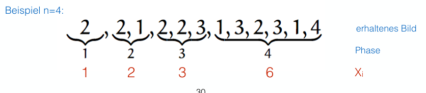
2.5.3,7 Coupon-Collector

Wenn es insgesamt $n$ “Sammelbilder” gibt, wie viele muss ich kaufen, bis ich alle besitze. Sei $X$ die Anzahl Runden, bis alle erhalten wurden.

Wir teilen den Prozess in $n$ Phasen. Phase $i$ ist die Anzahl Runden von $i - 1$ Coupons bis zum neuen Coupon $i$ . Sei $X_{i}$ die Anzahl Runden in Phase $i$ .

$X = X_{1} + X_{2} + \dots + X_{n}$
Linearität des Erwartungswertes: $E [X] = E [X_{1}] + \dots + E [X_{n}]$
In der Phase $i$ gilt: wir haben $i - 1$ unterschiedliche Coupons
Jede Runde ist die W’keit $1/ n$
es gibt $n - (i - 1) = n - i + 1$ Coupons die wir noch nicht haben
Dadurch gilt $p_{i} = \frac{n - i + 1}{n}$
Die Anzahl Runden ist dann $X_{i} \sim Geo (p_{i})$
Also gilt $E [X_{i}] = 1/ p_{i} = \frac{n}{n - i + 1}$ .

Dann ist $E [X] = \sum_{i = 1}^{n} E [X_{i}] = \sum_{i = 1}^{n} \frac{n}{n - i + 1}$ . Sei $k = n - i + 1$ , dann geht mit $i$ von $1 \to n$ , $k : n \to 1$ .
Dann gilt $E [X] = \sum_{k = 1}^{n} \frac{n}{k} = n \sum_{k = 1}^{n} \frac{1}{k} = n H_{n}$ wo $H_{n}$ die $n$ -te harmonische Zahl ist.

Wir wissen $H_{n} = ln n + O (1)$ und damit gilt $E [X] = n ln n + O (n)$ .

2.5.4 Poisson-Verteilung

Modelliert Menge an seltenen Ereignissen, während einer fixen Zeitspanne, wenn die Ereignisse mit konstanter Durschnittsrate und unabhängig auftreten. Example: Herzinfarkte in der Schweiz.

Wir definieren für eine Rate $λ = n p$ die die Verteilungsfunktion wie folgt

f_{X} (i) = {\frac{e ^{- λ} λ ^{i}}{i !} 0 f \overset{u}{¨} r i \in N_{0} sonst

Poisson EV and Var

Für $X \sim Po (λ)$ gilt
$E [x] = λ und Var [X] = λ$

Proof: We can derive both expectation and variance from the pmf using the explicit definitions:

E [X] = i = 0 \sum \infty k \cdot e^{- λ} \frac{λ ^{i}}{i !} = e^{- λ} \cdot i = 1 \sum i \frac{λ ^{i}}{i !} = e^{- λ} \cdot i = 1 \sum \frac{λ ^{i}}{( i - 1 )!} we reindex with j = i - 1 = e^{- λ} \cdot j = 0 \sum \frac{λ ^{j + 1}}{j !} = e^{- λ} \cdot λ \cdot j = 0 \sum \frac{λ ^{j}}{j !} = e^{- λ} \cdot λ \cdot e^{λ} = 1 \cdot λ

Poisson als Grenzwert der Binomialverteilung:
Another standard way to see the Poisson distribution is as “Balls and Bins”: we throw $n$ balls independently into $n$ bins. $X$ is the number of balls in the first bin.

For each the probability is $p = 1/ n$ , so $X \sim Bin (n, 1/ n)$
$E [X] = n \cdot (1/ n) = 1$
What happens to $Pr [X = i]$ as $n \to \infty$ ?
$Pr [X = i] = (i n) (1/ n)^{i} (1 - 1/ n)^{n - i}$ $= \frac{n ( n - 1 ) \dots ( n - i + 1 )}{i !} \frac{1}{n ^{i}} (1 - 1/ n)^{n - 1}$ $= \frac{n}{n} \frac{n - 1}{n} \dots \frac{n - i + 1}{n} \cdot \frac{1}{i !} \cdot (1 - 1/ n)^{n - 1}$
As $n \to \infty$
- $\frac{n - k}{n} \to 1$
- $(1 - 1/ n)^{n - 1} = (1 - 1/ n)^{n} \cdot (1 - 1/ n)^{- i} \to e^{- 1}$ as $(1 - 1/ n)^{- 1} = 1^{- i} = 1$
  Thus we get $lim_{n \to \infty} Pr [X = i] = \frac{e ^{- 1}}{i !}$

So more generally for $X \sim Bin (n, λ / n)$ , so $E [X] = λ$ , $lim_{n \to \infty} Pr [X = i] = \frac{λ ^{i} e ^{- λ}}{i !}$ .

2.6 Mehrere Zufallsvariablen

Für zwei Zufallsvariablen $X$ und $Y$ über demselben Wahrscheinlichkeitsraum schreiben wir

Pr [X = x, Y = y] := Pr [{ω \in Ω ∣ X (ω) = x, Y (ω) = y}]

Gemeinsame Dichte

Die Funktion
$f_{X, Y} (x, y) := Pr [X = x, Y = y]$
heisst gemeinsame Dichte der Zufallsvariablen $X$ und $Y$ .

Wir können aus der gemeinsamen Dichte wieder die Dichten der einzelnen Variablen ausrechnen:

Randdichte

Die Randdichte erhält man durch Summation über die jeweils andere Variable:

f_{X} (x) = y \in W_{Y} \sum f_{X, Y} (x, y), f_{Y} (y) = x \in W_{X} \sum f_{X, Y} (x, y)

Dies folgt direkt aus der totale Wahrscheinlichkeit, da die Ereignisse ${Y = y}$ eine disjunkte Zerlegung des Wahrscheinlichkeitsraums bilden.

Gemeinsame Verteilung

Die gemeinsame Verteilung zweier Zufallsvariablen $X$ und $Y$ ist
$F_{X, Y} (x, y) := Pr [X \leq x, Y \leq y] = x^{'} \leq x \sum y^{'} \leq y \sum f_{X, Y} (x^{'}, y^{'})$
Die Randverteilung ergibt sich als $F_{X} (x) = \sum_{x^{'} \leq x} \sum_{y \in W_{Y}} f_{X, Y} (x^{'}, y)$ .

Example: Skatblat: ziehe aus 32 Karten 10 Karten als Hand und 2 als Skat.
$X$ = Anzahl Buben in der Hand, $Y$ = Anzahl Buben im Skat. Gemeinsame Dichte:

Pr [X = x, Y = y] = \frac{( x 4 ) ( 10 - x 28 ) ( y 4 - x ) ( 2 - y 28 - ( 10 - x ) )}{( 10 32 ) ( 2 22 )}

Daraus folgt z.B. $Pr [X = 4, Y = 1] = 0$ , da es insgesamt nur 4 Buben gibt.

2.6.1 Unabhängigkeit von Zufallsvariablen

2.52 Unabhängigkeit

Zufallsvariablen $X_{1}, \dots, X_{n}$ heissen unabhängig genau dann, wenn für alle $(x_{1}, \dots, x_{n}) \in W_{X_{1}} \times \dots \times W_{X_{n}}$ gilt:
$Pr [X_{1} = x_{1}, \dots, X_{n} = x_{n}] = Pr [X_{1} = x_{1}] \dots Pr [X_{n} = x_{n}]$

Äquivalent: $f_{X_{1}, \dots, X_{n}} (x_{1}, \dots, x_{n}) = f_{X_{1}} (x_{1}) \dots f_{X_{n}} (x_{n})$ , d.h. für unabhängige Variablen ist die gemeinsame Dichte gleich dem Produkt der Randdichten.

Note, für $x_{i} \neq \in W_{x}$ gilt die Definition genauso, nur dass dann beide Seiten $0$ sind.

2.53 Produkteigenschaft für Mengen

Sind $X_{1}, \dots, X_{n}$ unabhängige Zufallsvariablen und $S_{1}, \dots, S_{n} \subseteq R$ beliebige Mengen, dann gilt
$Pr [X_{1} \in S_{1}, \dots, X_{n} \in S_{n}] = Pr [X_{1} \in S_{1}] \dots Pr [X_{n} \in S_{n}]$

Proof: Es genügt, $S_{i} \subseteq W_{X_{i}}$ zu betrachten. Dann:

Pr [X_{1} \in S_{1}, \dots, X_{n} \in S_{n}] = x_{1} \in S_{1} \sum \dots x_{n} \in S_{n} \sum Pr [X_{1} = x_{1}] \dots Pr [X_{n} = x_{n}] = (x_{1} \in S_{1} \sum Pr [X_{1} = x_{1}]) \dots (x_{n} \in S_{n} \sum Pr [X_{n} = x_{n}]) = Pr [X_{1} \in S_{1}] \dots Pr [X_{n} \in S_{n}]

2.54 Teilmengen bleiben unabhängig

Sind $X_{1}, \dots, X_{n}$ unabhängig und $I = {i_{1}, \dots, i_{k}} \subseteq [n]$ , dann sind $X_{i_{1}}, \dots, X_{i_{k}}$ ebenfalls unabhängig.

Intuitiv: sind $X_{1}, \dots, X_{n}$ unabhängig, so gilt dies auch für ${X_{1}, X_{7}, X_{3}}$ z.B.

Proof: Setze $S_{i} = W_{X_{i}}$ für $i \in / I$ und $S_{i} = {x_{i}}$ für $i \in I$ . Dann ist $X_{i} \in S_{i}$ für $i \in / I$ trivialerweise erfüllt und Lemma 2.53 liefert die Produktzerlegung:

Pr [X_{i_{1}} = x_{i_{1}}, \dots, X_{i_{k}} = x_{i_{k}}] = Pr [X_{1} \in S_{1}, \dots, X_{n} \in S_{n}] = Pr [X_{1} \in S_{1}] \dots Pr [X_{n} \in S_{n}] = Pr [X_{i_{1}} = x_{i_{1}}] \dots Pr [X_{i_{k}} = x_{i_{k}}]

Beachte, dass wir $Pr [X_{i} \in S_{i}]$ für $i \neq \in I$ im Produkt ignorieren können, da $Pr [X_{i} \in W_{X_{i}}] = 1$ gilt.

2.55 Funktionen unabhängiger Variablen

Seien $f_{1}, \dots, f_{n} : R \to R$ reellwertige Funktionen. Wenn $X_{1}, \dots, X_{n}$ unabhängig sind, dann sind auch $f_{1} (X_{1}), \dots, f_{n} (X_{n})$ unabhängig.

Proof: Für $z_{i} \in W_{f_{i} (X_{i})}$ definiere $S_{i} = {x ∣ f_{i} (x) = z_{i}}$ . Mit Lemma 2.53:

Pr [f_{1} (X_{1}) = z_{1}, \dots, f_{n} (X_{n}) = z_{n}] = Pr [X_{1} \in S_{1}, \dots, X_{n} \in S_{n}] = i = 1 \prod n Pr [X_{i} \in S_{i}] = i = 1 \prod n Pr [f_{i} (X_{i}) = z_{i}]

Beachte, Die Umkehrung gilt nicht: auch abhängige $X_{i}$ können nach Anwendung einer konstanten Funktion unabhängige Bilder haben. Siehe z.B. die konstante Funktion $f \equiv 1$ .

2.6.2 Zusammengesetzte Zufallsvariablen

Aus $X_{1}, \dots, X_{n}$ lässt sich durch eine Funktion $g$ eine neue Zufallsvariable $Y := g (X_{1}, \dots, X_{n})$ konstruieren. Die Wahrscheinlichkeiten berechnen sich wie gewohnt:

Pr [Y = y] = Pr [{ω ∣ g (X_{1} (ω), \dots, X_{n} (ω)) = y}]

2.58 Faltung / Konvolution unabhängige Zufallsvariablen $X$ und $Y$ sei $Z := X + Y$ . Dann gilt

Für zwei

$f_{Z} (z) = x \in W_{X} \sum f_{X} (x) \cdot f_{Y} (z - x)$

Intuitiv: Wir summieren über alle möglichen Paare basically.

Proof: Mit dem Satz von der totalen Wahrscheinlichkeit:

f_{Z} (z) = x \in W_{X} \sum Pr [X + Y = z ∣ X = x] \cdot Pr [X = x] = x \in W_{X} \sum Pr [Y = z - x] \cdot Pr [X = x]

Example: Poisson-Stabilität: Sind $X \sim Poisson (λ_{X})$ und $Y \sim Poisson (λ_{Y})$ unabhängig, so gilt mit dem Binomialsatz:

f_{Z} (z) = e^{- (λ_{X} + λ_{Y})} \cdot \frac{( λ _{X} + λ _{Y} ) ^{z}}{z !}

d.h. $Z = X + Y \sim Poisson (λ_{X} + λ_{Y})$ . Die Poisson-Verteilung ist stabil unter Faltung.

2.6.3 Momente zusammengesetzter Zufallsvariablen

2.60 Linearität des Erwartungswerts

Für Zufallsvariablen $X_{1}, \dots, X_{n}$ (beliebig, auch abhängig) und $X := a_{1} X_{1} + \dots + a_{n} X_{n}$ mit $a_{i} \in R$ gilt
$E [X] = a_{1} E [X_{1}] + \dots + a_{n} E [X_{n}]$

Beachte, damit oberes gilt, müssen die Zufallsvariablen nicht unabhängig sein!

2.61 Multiplikativität des Erwartungswerts

Für unabhängige Zufallsvariablen $X_{1}, \dots, X_{n}$ gilt
$E [X_{1} \dots X_{n}] = E [X_{1}] \dots E [X_{n}]$

Proof: Basisfall $n = 2$ . Mit der Unabhängigkeit:

E [X \cdot Y] = x \in W_{X} \sum y \in W_{Y} \sum x y \cdot Pr [X = x, Y = y] = x \in W_{X} \sum y \in W_{Y} \sum x y \cdot Pr [X = x] Pr [Y = y] = (x \sum x Pr [X = x]) (y \sum y Pr [Y = y]) = E [X] E [Y]

Wobei dank Unabhängigkeit $Pr [X = x, Y = y] = P r [X = x] \cdot Pr [Y = y]$ hält.

Beachte, die Unabhängigkeit ist notwendig: für $Y = X$ gilt $E [X^{2}] \neq = (E [X])^{2}$ im Allgemeinen (sonst gilt Varianz = 0).

2.62 Varianz der Summe

Für unabhängige Zufallsvariablen $X_{1}, \dots, X_{n}$ und $X := X_{1} + \dots + X_{n}$ gilt
$Var [X] = Var [X_{1}] + \dots + Var [X_{n}]$

Proof: Basisfall $n = 2$ , $Z = X + Y$ .

Berechne $E [(X + Y)^{2}]$ und $E [X + Y]^{2}$ und subtrahiere.
Unabhängigkeit liefert $E [X Y] = E [X] E [Y]$ , wodurch sich die gemischten Terme aufheben

E [(X + Y)^{2}] - E [X + Y]^{2} = (E [X^{2}] - E [X]^{2}) + (E [Y^{2}] - E [Y]^{2}) = Var [X] + Var [Y]

Für abhängige Variablen gilt die Formel im Allgemeinen nicht. Gegenbeispiel: $Y = - X$ $\Rightarrow$ $Var [X + Y] = 0 \neq = 2 Var [X]$ ).

Varianz eines Produktes

Beachte, für Produkte gilt selbst bei Unabhängigkeit nicht allgemein, dass $Var [X Y] = Var [X] Var [Y]$ .

Zusammenfassung

Property	Always True?	Conditions Required
$E [X + Y] = E [X] + E [Y]$	✅ Always	None
$E [X Y] = E [X] \cdot E [Y]$	✅ If independent	$X, Y$ independent
$Va r [X + Y] = Va r [X] + Va r [Y]$	✅ If independent	$X, Y$ (pairwise) independent
$Va r [X Y] = Va r [X] \cdot Va r [Y]$	❌ Not in general	Fails even if independent

2.6.4 Waldsche Identität

In vielen Anwendungen ist die Anzahl der Summanden selbst eine Zufallsvariable (z.B. Laufzeit eines Algorithmus, der eine zufällige Anzahl Phasen durchläuft).

Waldsche Identität (Satz 2.65)

Seien $N$ und $X$ unabhängige Zufallsvariablen mit $W_{N} \subseteq N$ , und sei $Z := \sum_{i = 1}^{N} X_{i}$ wobei $X_{1}, X_{2}, \dots$ unabhängige Kopien von $X$ sind. Dann gilt
$E [Z] = E [N] \cdot E [X]$

Proof: Mit dem Satz von der totalen Wahrscheinlichkeit und der Linearität:

E [Z] = n \in W_{N} \sum E [Z ∣ N = n] \cdot Pr [N = n] = n \in W_{N} \sum n \cdot E [X] \cdot Pr [N = n] = E [X] \cdot E [N]

Der entscheidende Schritt ist $E [Z ∣ N = n] = E [X_{1} + \dots + X_{n}] = n E [X]$ (Linearität, da $n$ jetzt eine Konstante ist).

Example: Eine Münze mit Kopf-Wahrscheinlichkeit $p$ wird so lange geworfen, bis das erste Mal Kopf erscheint ( $N \sim Geom (p)$ , $E [N] = 1/ p$ ).
Dann wird $N$ -mal weitergeworfen, $Z$ = Anzahl Kopf. Die Waldsche Identität liefert direkt $E [Z] = \frac{1}{p} \cdot p = 1$ .

2.6.Exkurs Bedingte Zufallsvariablen

Bedingte Zufallsvariablen

Sei $X$ eine Zufallsvariable und $A \subset Ω$ ein Ereigniss.
Dann gilt
$Pr [X ∣ A = x] = Pr [X = x ∣ A]$

Wir wollen also nur die Wahrscheinlichkeit von $X = x$ , gegeben dass $A$ Eintritt, wissen.

Es gilt dann genauso wie für Ereignisse der Satz der totalen W’keit:

Satz der totalen W'keit (ZV)

Für $A_{1}, \dots, A_{n}$ disjunkt mit $A_{1} \cup \dots \cup A_{n} = Ω$ und $Pr [A_{1}], \dots, Pr [A_{n}] > 0$ gilt
$E [X] = i = 1 \sum n E [X ∣ A_{i}] \cdot Pr [A_{i}]$

Proof:

E [X] = α \in W_{x} \sum α \cdot Pr [X = α] = α \in W_{x} \sum α \cdot i = 1 \sum n Pr [X = α ∣ A_{i}] \cdot Pr [A_{i}] = i = 1 \sum n Pr [A_{i}] \cdot α \in W_{x} \sum α \cdot Pr [X = α ∣ A_{i}] = i = 1 \sum n Pr [A_{i}] \cdot E [X ∣ A_{i}]

where the first inequality follows directly from the Satz der totalen W’keit.

2.7 Abschätzen von Wahrscheinlichkeiten

Der Erwartungswert einer ZV kann stark von dem erwarteten Ergebnis für einen einzigen Wurf abweichen (z.B. ZV die mit sehr kleiner chance sehr großen Wert annimmt).

2.7.1 Die Ungleichungen von Markov und Chebychev

2.67 Markov-Ungleichung

Sei $X$ eine Zufallsvariable mit $X \geq 0$ (nicht-negativ). Dann gilt für alle $t > 0$ :
$Pr [X \geq t] \leq \frac{E [ X ]}{t}$
Äquivalent: $Pr [X \geq t \cdot E [X]] \leq \frac{1}{t}$ .

Proof:

E [X] = x \in W_{x} \sum x \cdot Pr [X = x] \geq x \in W_{x}, x > t \sum x \cdot Pr [X = x] \geq t \cdot x \in W_{x}, x > t \sum Pr [X = x] = t \cdot Pr [X \geq t]

Die Ungleichung ergibt sich im wesentlichen durch das Weglassen einiger Summanden (denen mit $x \leq t$ ).

Wenn wir die Markov-Ungleichung auf die Varianz anstatt den Erwartungswert anwenden, erhalten wir die Chebychev-Ungleichung.

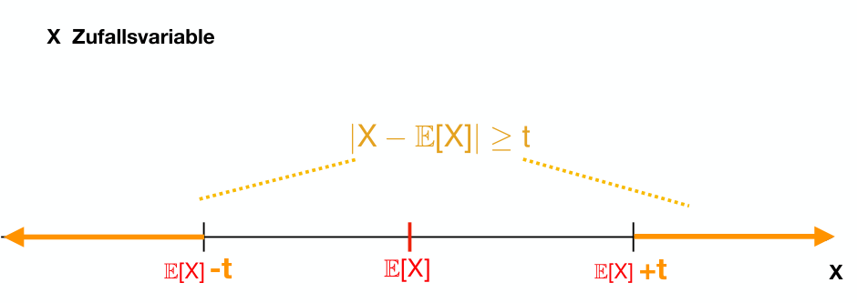
2.68 Chebyshev-Ungleichung

Sei $X$ eine Zufallsvariable und $t > 0$ . Dann gilt
$Pr [∣ X - E [X] ∣ \geq t] \leq \frac{Var [ X ]}{t ^{2}}$
Äquivalent: $Pr [∣ X - E [X] ∣ \geq t Var [X]] \leq \frac{1}{t ^{2}}$ .

Proof: Es gilt

Pr [∣ X - E [X] ∣ \geq t] = Pr [(X - E [X])^{2} \geq t]

dies folgt da wir immer die Ungleichung innerhalb des $Pr [\dots]$ manipulieren können und $∣ X - E [X] ∣ \geq t ⟺ (X - E [X])^{2} \geq t^{2}$ .

Die ZV $Y = (X - E [X])^{2}$ ist nicht-negativ und $E [Y] = Var [X]$ (da $Var [X] = E [(X - E [X])^{2}] = E [Y]$ ).
Durch anwenden der Markov-Ungleichung kommen wir dann zu:

Pr [∣ X - E [X] ∣ \geq t] = Pr [Y \geq t^{2}] \leq \frac{E [ Y ]}{t ^{2}} = \frac{Var [ X ]}{t ^{2}}

Intuitiv, je kleiner die Varianz, desto größer ist die W’keit dass $X$ nur Werte innerhalb eines Intervalls $[E [X] - t, E [x] + t]$ annimmt.
Je kleiner die Varianz, desto konzentrierter ist $X$ um seinen Erwartungswert.

Example: Coupon-Collector: Sei $X$ die Anzahl Käufe beim Coupon-Collector-Problem mit $n$ Bildern. Es gilt $E [X] = n H_{n}$ und $Var [X] \leq n^{2} \cdot \frac{π ^{2}}{6}$ . Chebyshev liefert für $f (n) = n ln n$ :

Pr [∣ X - E [X] ∣ \leq n ln n] \geq 1 - \frac{π ^{2}}{6 ln n}

2.7.2 Die Ungleichung von Chernoff

Wenn wir mehr über die Verteilung wissen, können wir bessere Schranken erreichen, als nur die Markov- und Chebychev-Ungleichungen.
Für Summen von Bernoulli-Variablen gibt es wesentlich schärfere Schranken:

2.70 Chernoff-Schranken

Seien $X_{1}, \dots, X_{n}$ unabhängige Bernoulli-Variablen mit $Pr [X_{i} = 1] = p_{i}$ , und sei $X := \sum_{i = 1}^{n} X_{i}$ . Dann gilt:
$(i) Pr [X \geq (1 + δ) E [X]] \leq e^{- \frac{1}{3} δ^{2} E [X]} f \overset{u}{¨} r alle 0 < δ \leq 1$ $(ii) Pr [X \leq (1 - δ) E [X]] \leq e^{- \frac{1}{2} δ^{2} E [X]} f \overset{u}{¨} r alle 0 < δ \leq 1$ $(iii) Pr [X \geq t] \leq 2^{- t} f \overset{u}{¨} r t \geq 2 e E [X]$

Proof: iii) Wende die Markov-Ungleichung auf $Y = 4^{X}$ an (streng monoton, also ${X \geq t} = {4^{X} \geq 4^{t}}$ ).
Mit:

der Unabhängigkeit und Satz 2.55 (Funktion von unabhängigen sind wieder unabhängig) sind $4^{X_{i}}$ unabhängig
Satz 2.61 (Erwartung ist Multiplikativ für unabhängige) liefert:

E [4^{X}] = i = 1 \prod n E [4^{X_{i}}] = i = 1 \prod n (1 + 3 p_{i}) \leq i = 1 \prod n e^{3 p_{i}} = e^{3 E [X]}

Für $t \geq 2 e E [X]$ gilt $e^{3 E [X]} \leq 2^{t}$ , woraus $Pr [X \geq t] \leq \frac{E [ 4 ^{X} ]}{4 ^{t}} \leq \frac{2 ^{t}}{4 ^{t}} = 2^{- t}$ folgt. Die Teile (i) und (ii) folgen analog mit $Y = (1 \pm δ)^{X}$ .

2.8 Randomisierte Algorithmen

Ein normaler Algorithmus, geschrieben als $A (I)$ gibt für den gleichen Input immer den gleichen Output aus.
Einem randomisierten Algorithmus stellen wir außerdem noch Zufall, in der Form von $n$ -Zufallsbits $R$ zur Verfügung, geschrieben als $A (I, R)$ .

Monte-Carlo Algorithmus

Für einen Monte-Carlo Algorithmus gilt, dass:

die Korrektheit eine ZV ist

Laufzeit fix ist

Immer schnell, mit meistens richtiger Antwort.

Las-Vegas Algorithmus

Für einen Las-Vegas Algorithmus gilt, dass:

die Ausgabe immer Korrekt ist (nicht vom Zufall abhängt)

Die Laufzeit eine ZV ist

Immer richtig, jedoch nur meistens schnell.

Alternative Definition: Las-Vegas:
Wir können einen Las-Vegas Algorithmus auch ??? ausgeben lassen, wenn er sich nicht sicher ist. Dies wäre auch eine “korrekte” Ausgabe. Die Garantie ist dann: “wenn die Antwort nicht ??? ist, ist sie korrekt”.
Arten von LV-Algos:

Wiederholen bis nicht mehr ??? rauskommt
Für $T$ laufen lassen, wenn bis dahin nichts kommt dann ???

Note, wir können jeden LV-Algo in einen ??? LV-Algo konvertieren, in dem wir in fix $T$ laufen lassen, und dann aborten. Falls er JA/NEIN zurückgegeben hat das ausgeben, sonst ???.

2.8.1 Reduktion der Fehlerwahrscheinlichkeit

2.72 Las-Vegas-Fehlerreduktion

Sei $A$ ein randomisierter LV-Algorithmus mit $Pr [A (I) korrekt] \geq ε$ .
Dann gilt für den Algorithmus $A_{δ}$ , der $A$ bis zu $N = ε^{- 1} ln δ^{- 1}$ mal wiederholt (und bei der ersten Nicht-???-Antwort abbricht):
$Pr [A_{δ} (I) korrekt] \geq 1 - δ$

Note, $Pr [A (I) korrekt] \geq ϵ$ heißt, dass der Algorithmus maximal mit W’keit $1 - ϵ$ ??? ausgibt.

Proof: Die Wahrscheinlichkeit, dass alle $N$ Aufrufe ??? liefern, ist $\leq (1 - ε)^{N}$ $\leq e^{- εN} = e^{l n δ} = δ$ .

Für einen MC-Algo ist die Reduktion der Fehler-W’keit nicht ganz so einfach. Er muss eine der folgenden Bedingungen erfüllen:

Der Algorithmus hat einen einseitigen Fehler.
$Pr [A (I) korrekt] > 1/2$ (besser als Zufall) (zweiseitiger Fehler)

2.74 Monte-Carlo mit einseitigem Fehler

Sei $A$ ein Algorithmus mit $Pr [A (I) = Ja] = 1$ für Ja-Instanzen und $Pr [A (I) = Nein] \geq ε$ für Nein-Instanzen.
Der Algorithmus $A_{δ}$ wiederholt bis zum ersten Nein (maximal $N = ε^{- 1} ln δ^{- 1}$ mal). Dann gilt:
$Pr [A_{δ} (I) korrekt] \geq 1 - δ$

Wenn der Algorithmus also bei “Ja-Instanzen” immer korrekt “Ja” ausgibt, hat er einen einseitigen Fehler. Wir wiederholen also bis entweder “Ja” kommt (dann ist sicher “Ja” richtig) oder “Nein” sehr wahrscheinlich wird.

2.75 Monte-Carlo mit zweiseitigem Fehler

Sei $Pr [A (I) korrekt] \geq \frac{1}{2} + ε$ .
Der Algorithmus $A_{δ}$ macht $N = 4 ε^{- 2} ln δ^{- 1}$ unabhängige Aufrufe und gibt die Mehrheitsantwort aus. Dann gilt:
$Pr [A_{δ} (I) korrekt] \geq 1 - δ$

Proof: Sei $X$ die Anzahl korrekter Antworten.

$X \sim Binomial (N, \frac{1}{2} + ϵ)$
1. Es gilt $E [X] = pN \geq \frac{N}{2} + εN$
2. durch sehr viel handwaving gilt $\frac{N}{2} \leq (1 - ε) E [X]$ .
Wir wollen begrenzen $Pr [A_{δ} (I) ist inkorrekt] = Pr [X \leq N /2]$ als kleiner als $δ$ .
Chernoff (ii) $Pr [X \leq (1 - ϵ) E [X]] \leq e^{- ϵ^{2} E [X] /2}$
1. von vorher wissen wir das gilt $\frac{N}{2} \leq (1 - ϵ) E [X]$
2. also $Pr [X \leq N /2] \leq e^{- \frac{1}{2} ε^{2} E [X]}$ .
Da $\frac{N}{2} \leq (1 - ϵ) E [X]$ gilt auch $\frac{N}{2} \leq E [X]$ weil $1 - ϵ < 1$ .
1. Also gilt $Pr [X \leq N /2] \leq e^{- \frac{1}{4} ε^{2} N}$
und wir wollen $e^{- \frac{1}{4} ε^{2} N} \geq δ$
1. $N \geq \frac{4}{ϵ ^{2}} ln (\frac{1}{δ})$
  Deswegen müssen wir $N = ⌈ \frac{4}{ϵ ^{2}} ln (\frac{1}{δ}) ⌉$ wählen.

2.76 Fehlerreduktion für Optimierungsprobleme

Sei $Pr [A (I) \geq f (I)] \geq ε$ .
Der Algorithmus $A_{δ}$ macht $N = ε^{- 1} ln (δ^{- 1})$ Aufrufe und gibt das Beste zurück. Dann gilt $Pr [A_{δ} (I) \geq f (I)] \geq 1 - δ$ .

Proof: Die W’keit das bei $N$ Aufrufen kein einziges Mal $\geq f (I)$ kommt ist höchstens

(1 - ϵ)^{N} \leq e^{- ϵ N} = e^{- l n δ^{- 1}} = δ

wir benutzen $1 + x \leq e^{x}$ und $- l n (1/ δ) = l n ((1/ δ)^{- 1}) = l n (δ)$ .

2.8.2 Sortieren und Selektieren

We know that for a worst-case input (inversely sorted list), when always choosing the last element as a pivot, quicksort needs $O (n^{2})$ time (as each partition splits off 1 element).

This randomised Quicksort procedure has $O (n ln n)$ expected runtime.

By randomly choosing the pivot element, we can reduce this to $O (n lo g n)$ on average. That is we want to show that

E [T_{1, n}] \leq 2 (n + 1) ln + O (n)

Let $T_{l, r}$ be the number of comparisons. For $l \geq r$ $T_{l, r} = 0$ . For $l < r$ we have recursively

E [T_{l, r}] = i = l \sum r Pr [t = i] \cdot (r - l + E [T_{l, i - 1}] + E [T_{i + 1, r}])

by assumption all elements are unique. Thus $Pr [t = i] = \frac{1}{r - l + 1}$ , as each is equally likely to be chosen. We notice $E$ does not depend on $l$ or $r$ , but only on the length $r - l + 1$ .

Then we define

t_{n} = {0, \frac{1}{n} \sum_{i = 0}^{n} (n - 1 + t_{i} + t_{n - i + 1}) falls n \leq 1, und

for easier handling.
Then for $n \geq 3$ we have $n \cdot t_{n} = \sum_{i = 0}^{n - 1} (n - 1 + t_{i} + t_{n - i - 1})$ and $(n - 1) \cdot t_{n - 1} = \sum_{i = 0}^{n - 2} (n - 2 + t_{i} + t_{n - i - 2}$ .
By subtracting we get

n t_{n} - (n - 1) t_{n - 1} = 2 (n - 1) + 2 t_{n - 1}

and thus

t_{n} = \frac{n + 1}{n} \cdot t_{n - 1} + \frac{2 ( n - 1 )}{n} \leq \frac{n + 1}{n} t_{n - 1} + 2

By using induction $t_{n} \leq 2 \sum_{i = 3}^{n + 1} \frac{n + 1}{i}$ . We can factor out the $n + 1$ and then we get the harmonic sequence (which is $O (ln n) + O (1)$ . Thus

E [T_{1, n}] = t_{n} \leq 2 (n + 1) ln n + O (n)

as $\sum_{i = 1}^{n} \frac{1}{i} = H_{n} = ln n + O (1)$ .

We also look at Quickselect: it has $O (n)$ linear runtime.

Quickselect allows us to find the k-th smallest element in an array. It does this without sorting, by partitioning the array and choosing the part in which the k-th smallest must then be.
This has linear $O (n)$ runtime, which we want to prove:

We define a random sequence $(l_{0}, r_{0}, k_{0}), (l_{1}, r_{1}, k_{1}), \dots, (l_{N}, r_{N}, k_{N})$ which defines the sequence of $N$ partitioning choices we make to find the target element.
From the algorithm we see that by construction $(l_{0}, r_{0}, k_{0}) = (1, n, k)$ and that $(l_{i + 1}, r_{i + 1}) = (l_{i}, t - 1) or (t + 1, r_{i})$ .

Then the number of comparisons for a call of Quicksort is $T = \sum_{i = 1}^{N} (r_{i} - l_{i})$ as each call does exactly $r_{i} - l_{i}$ comparisons.

We now want to bound the total number of comparisons. We do this by sorting them into buckets, each $3/4$ of the remaining elements.
We define $N_{j}$ as the number of calls for which $\frac{3}{4}^{j} n < r_{i} - l_{i} + 1 \leq \frac{3}{4}^{j - 1} n$ .

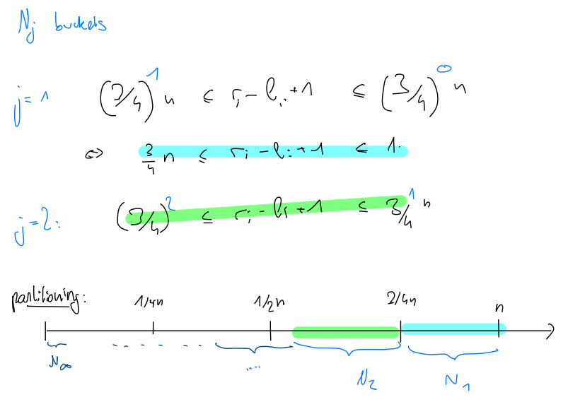
Since $(3/4)^{j - 1} n$ is the upper bound for each call in $N_{j}$ , we know

T \leq j = 1 \sum \infty N_{j} \cdot (\frac{3}{4})^{j - 1} n

By the linearity of expectation

E [T] \leq n \cdot j = 1 \sum \infty E [N_{j}] \cdot (\frac{3}{4})^{j - 1}

what do we know about $E [N_{j}]$ ? If the pivot is chosen in the middle half of the array, then $(l_{i}, t - 1)$ or $(t + 1, r_{i})$ are smaller than $3/4 \cdot (l_{i}, r_{i})$ . As it’s uniform, the probability of that happening is $1/2$ . Thus $E [N_{j}] = \frac{1}{\frac{1}{2}} = 2$ .
Therefore

E [T] \leq 2 n j = 1 \sum \infty (\frac{3}{4})^{j - 1} = 8 n

Note: for a practical implementation where there can be non-distinct integers, we need tripartition using the “dutch flag algorithm” for in place partitioning into <, ==, >.
https://leetcode.com/problems/kth-largest-element-in-an-array

2.8.3 Miller-Rabin-Primzahlentest

For RSA or other crypographic applications, we often need primes of multiple thousands of bits. Usual procedure: choose random number of that length → check if prime.
Naively, this can be done by checking all numbers $< n$ . But this is very inefficient for such large numbers (imagine 4096 bits).

We want an algorithm that is polynomial in $l n (n)$ , (so polynomial with regards to the number of digits, i.e. in $lo g_{10} n$ ).

Naive approach Choose randomly, check for certificates

we choose a random number in $a \in {2, \dots, n}$
check if $g cd (a, n) > 1$ .
If yes, we found a certificate for the non-primality of $n$ .
(This is an example of a las-vegas algorithm with a one-sided error.)

This does not work well for numbers $n = pq$ a composite of two prime numbers. Then the chance we find one of them is $\approx 1/ n$ , so we need $O (n)$ to find one.

Using Fermat We know from diskmath that if $n \in N$ prime, then $\forall a \in N, 0 < a < n$

a^{n - 1} \equiv_{n} 1

(Fermat’s little theorem).
So if we find an $a$ s.t. $a^{n - 1} \neq \equiv_{n} 1$ , then we know for sure that $n$ is not prime.
Note: we can exponentiate efficiently using binary exponentiation.

Carmichael Numbers: There are numbers that are not prime, but for all $a$ s.t. $g cd (a, n) = 1$ satisfy $a^{n - 1} \equiv_{n} 1$ . The smallest such number is $561 = 3 \cdot 11 \cdot 17$ .

thus we don’t find any certificates we wouldn’t already find by computing the gcd for a large number of random $a$ .
As there are an infinite amount of these Carmichael numbers, we still have to refine our approach.
→ See Why are there Carmichael Numbers.

Miller-Rabin:

if $n$ prime, $0 \leq a < n$ for a field with addition and multiplication.
We take $x^{2} \equiv_{n} 1$
- $⟹ x^{2} - 1 \equiv_{n} 0 ⟹ (x + 1) (x - 1) \equiv_{n} 0$
- In a field, there are no zero-divisors
- Thus $(x + 1) (x - 1) = 0$ iff. $x = \pm 1$ ( $x = 1$ or $x = n - 1$ )
We can use this to our advantage. If we find an $x$ satisfying this with $x \neq = \pm 1$ , we know there is a zero-divisor $⟹$ $Z_{n}$ not a field $⟹$ $n$ not prime

We incorporate this into the algorithm in the following way.

we write $n - 1 = d 2^{k}$ where $d$ odd (i.e. choose the biggest $k$ possible)
if $n$ prime, $a^{n - 1} \equiv_{n} (a^{d})^{2^{k}} \equiv_{n} 1$
- Therefore $(a^{d})^{2^{k - 1}} \equiv \pm 1$ (or $n - 1$ ) as proven before
We iterate over $k$ .
- Either for all $0 \leq i \leq k$ $(a^{d})^{2^{i}} \equiv_{n} 1$
- or there is an $0 \leq i \leq k - 1$ s.t. $(a^{d})^{2^{i}} \equiv_{n} n - 1$
if both conditions are violated, $n$ is not prime and we found our certificate $a$ .
- intuitively: if we find an $i$ with $0 \leq i < k$ s.t. $b = (a^{d})^{2^{i}} \neq \equiv \pm 1$ and $b^{2} = (a^{d})^{2^{i + 1}} \equiv_{n} 1$ then we found a $b \in Z_{n}$ with $b^{2} \equiv 1$ for $b \neq = \pm 1$ → $Z_{n}$ not a field.

In other words, the chain of numbers $b_{0} \to b_{1} \to \dots \to b_{n}$ we get when running the algorithm can be

$1 \to 1 \to \dots \to 1$
$- 1 \to 1 \to \dots \to 1$
$\neq = \pm 1 \to \neq = \pm 1 \to \dots \to - 1 \to 1$
But never have $\neq = \pm 1 \to 1$ in it
Why can we have $\neq = \pm 1 \to - 1$ ? because $x^{2} \equiv_{n} - 1 ⟹ x^{2} + 1 \equiv_{n} 0$ and there is nothing that forbids this.
$5$ is prime yet $2^{2} \equiv_{5} 4 \equiv_{5} - 1$

Example: $n = 97$ so $n - 1 = 96 = d 2^{k}$ with $d = 3$ and $k = 5$ .

$b_{0} = 5^{3} \equiv_{n} 28$
$b_{1} = 2 8^{2} \equiv_{n} 8$
…
$b_{4} = 2 2^{2} \equiv_{n} - 1$
$b^{5} = (- 1)^{2} \equiv_{n} 1$
which is a valid chain. Thus 97 is prime

2.8.4 Target-Shooting

Gegeben einer Menge $U$ und einer Untermenge $S \subseteq U$ unbekannter Größe, wie groß ist $∣ S ∣/∣ U ∣$ . Wir nehmen an wir haben für $S$ die Indikatorfunktion $I_{S} : U \to 0, 1$ (we need $I_{S}$ efficiently computable).

Algorithmus: Für $N > 0$ geeignete Wahl, wähle $N$ Elemente auf $U$ zufällig aus und return $found / N$ zurück: $N^{- 1} \cdot \sum_{i = 1}^{N} I_{S} (u_{i})$ .

Let $Y_{i} := I_{S} (u_{i})$ . Because of uniform and independent choice of $u_{i}$ , the random variables $Y_{1}, \dots, Y_{n}$ are independent Bernoulli variables with $Pr [Y_{i} = 1] = ∣ S ∣/∣ U ∣$ .
Thus

Y := \frac{1}{N} i = 1 \sum N Y_{i} = \frac{1}{N} i = 1 \sum N I_{S} (u_{i})

Therefore $E [Y] = ∣ S ∣/∣ U ∣$ , as $E [Y_{i}] = ∣ S ∣/∣ U ∣$ , independent of the choice of $N$ . The variance:

Var [Y] = \frac{1}{N} (\frac{∣ S ∣}{∣ U ∣} - (\frac{∣ S ∣}{∣ U ∣})^{2})

is dependent on $N$ however.

Let $ϵ > 0$ . How large must $N$ be for the algorithm to return an answer in $[(1 - ϵ) \frac{∣ S ∣}{∣ U ∣}, (1 + ϵ) \frac{∣ S ∣}{∣ U ∣}]$ with probability $1/2$ ?

Target Shooting

Let $δ, ϵ > 0$ . If $N > 3 \frac{∣ U ∣}{∣ S ∣} \cdot ϵ^{- 2} \cdot ln (2/ δ)$ then the returned value is within
$[(1 - ϵ) \frac{∣ S ∣}{∣ U ∣}, (1 + ϵ) \frac{∣ S ∣}{∣ U ∣}]$
with probability at least $1 - δ$ .

Proof:

Because $E [Y] = \frac{∣ S ∣}{∣ U ∣}$ it suffices to show

Pr [∣ Y - E [Y] ∣ \geq ϵ \cdot E [Y]] \leq δ

we note $Z := \sum_{i = 1}^{N} Y_{i} = N Y$ , this is equivalent to $Pr [∣ Z - E [Z] ∣ \geq ϵ \cdot E [Z]] \leq δ$
As $Y_{i}$ are independent bernoulli variables, we can use the chernoff bounds:

Pr [∣ Z - E [Z] ∣ \geq ϵ \cdot E [Z]] \leq 2 e^{- ϵ^{2} E [Z] /3} = 2 e^{- ϵ^{2} N ∣ S ∣/ (3∣ U ∣)}

2.8.5 Finden von Duplikaten

Lecture 8: Hashing with Chaining (MIT OCW)
Lecture 9: Table Doubling, Karp-Rabin (MIT OCW)
Lecture 10: Open Addressing, Cryptographic Hashing (MIT OCW)

Lecture 8: Randomization: Universal & Perfect Hashing

— TODO: Update with notes from “Algorithmen” book about hashing types (p. 253)

see chaining vs. open addressing
universal hash functions

How do we find duplicates in an array?
Naive approaches

we could sort the array in $O (n lo g n)$
and check for duplicates by scanning again in $O (n)$
For collecting all duplicate pairs, we will then need $∣ Dupl (D) ∣$ time. Thus total complexity $O (n lo g n + ∣ Dupl (D) ∣)$ .

However, some real world constraints might be that the elements in the array are large (files for example) that we can’t simply sort. Memory accesses and comparisons are very slow in that case.

We can use hash-functions in this case. A hash-function needs to be efficiently computable and uniformly distribute the elements, i.e. $Pr [h (u) = i] = 1/ m$ for all $u \in U$ .

We can now solve the problem by adding each element to the hashmap and counting the duplicates at the end:

for each element $s_{k}$ , hash and create pair $(h (s_{k}), k)$
sort them by hash
iterate through the sorted list. If $(h (s_{i}^{'}), idx_{i}^{'})$ and $(h (s_{j}^{'}), idx_{j}^{'})$ have $h (s_{i}^{'}) = h (s_{j}^{'})$ then we have our candidate duplicate pair
For each pair, we perform a full comparison.

To estimate the runtime, we need to calculate the expected number of collisions:

For $X_{i}$ $1$ iff. there is a collision $s_{j}$ with $s_{i} \neq = s_{j}$ . Then $Pr [X_{i} = 1] = 1 - (1 - \frac{1}{m})^{n - 1}$
- this is because each element is mapped to a uniformly random value in the $[m]$ bits and there are $n - 1$ other values.
- Thus $(1 - 1/ m)$ is the probability of hashing to a different value. We do it $n - 1$ times to get the prob that all hash to a different value
- Then $1 -$ that to find the prob that there is at least 1 collision
Thus $E [# collisions] \leq Number of duplicates + \sum_{i = 1}^{n} E [X_{i}]$ $\leq number of duplicates + n \cdot (1 - (1 - \frac{1}{m})^{n - 1})$
If we choose $m$ such that $1 - (1 - 1/ m)^{n - 1} = O (\frac{1}{n})$ holds, we’ll only expect an $O (1)$ number of collisions.

Therefore the hashmap duplicate counter takes only $Θ (n lo g n)$ time, for the sorting of the hashmap.

2.8.6 Bloom Filters

https://samwho.dev/bloom-filters

Bloom filters are a probabilistic data structure. They have a one-sided error. They

can give false positives
but never false negatives.

It does this by using $n$ bits and $k$ hash functions. On insertion, we set $k$ bits, one for each hash function. To check if the filter contains an element, we check if those bits are set (this might return a false positive). We cannot delete however.

Estimating the probability of false positives: A false positive occurs when $s_{i}$ was not previously inserted but $M [x_{1}] = \dots = M [x_{k}] = 1$ (where $M [x_{i}]$ is the bit set by hashing $s$ with hash function $i$ ).
Let $X_{i} = 1$ if $s_{j}$ is a false positive, otherwise 0. We want to estimate $E [# false entries in L] = \sum_{j = 1}^{n} E [X_{j}]$ . Let $m$ be the number of bits in the bloom filter.

Suppose $l$ items have been inserted before processing $s_{j}$ . Each item set $k$ bits. So in total, up to $k l$ bits might be set.
$Pr [M [x] = 0] = (1 - \frac{1}{m})^{k l} \approx 1 - e^{- k l / m}$ (probability bit not set $= 1 - 1/ m$ and that for $k l$ repetitions)
Then for $s_{j}$ , the probability that all $k$ hash bits are $1$ is $Pr [X_{j} = 1] \approx (1 - e^{- k l / m})^{k}$ .
Worst case $l = j - 1 \approx n$ . And as each bit is independent, the sum can be collapsed to $\cdot n$ . Therefore

E [# false positives] \leq n \cdot (1 - e^{kn / m})^{k}

So the false positive rate is minimised for $k = \frac{m}{n} ln 2$ . If we want to minimise the false positives, we choose $k = ln n$ and $m = n ln n$ .

Counting Bloom Filters By instead counting the number of times a certain bit has been activated, we can make removal possible.

this introduces the possibility of false negatives however
if add(a) set bit 0, 1 and add(b) set bit 2, 3. then remove(c) unsets 1, 2 → even though c was never added, it removed something. Now if find(a) is called it will return a false negative.

Extra

Why are there Carmichael Numbers

For a group $G$ there is

the order $∣ G ∣$ the number of elements
the order $ord (a)$ of each element $a \in G$ .
Lagrange tells us that $\forall a, ord (a) ∣ ∣ G ∣$ .
For cyclic groups, these coincide:
see $Z_{5}$ where $1^{4} = 1, 2^{4} = 1, 3^{4} = 1, 4^{4} = 1$ .

For a squarefree $n = p_{1} p_{2} \dots p_{k}$ , we have $Z_{n} ≅ Z_{p_{1}} \times Z_{p_{2}} \dots Z_{p_{k}}$
It’s generally not cyclic, it’s a direct product. Now, the order and the order/exponent diverge:

Order $:= ϕ (n)$
order of each element $= lcm (p_{i} - 1)$
- aside: why lcm? because $(a_{1}, a_{2}, \dots, a_{k}) \in Z_{n}$ needs to hit $(e, e, \dots, e)$ simultaneously. So the exponent has to be the lcm of the individual orders.
  For $n = 561 = 3 \times 11 \times 17$ , the order of each component is $(2, 10, 16)$ , thus the product has $2 \times 10 \times 16 = 320$ but the lcm is $lcm (2, 10, 16) = 80$ .
  Thus every element satisfies $g^{80} = 1$

And because $n - 1 = 560 = 80 \times 7$ , $a^{560} = (a^{8} 0)^{7} = 1^{7} = 1$ for all numbers. Thus $561$ is a Carmichael.

Niklas @ ETHZ

Explorer

2. Wahrscheinlichkeitstheorie

2.0 Intro

2.0.1 Ordered Selection with Replacement - Tuples

2.0.2 Ordered Selection without Replacement - k-Permutations

2.0.3 Unordered Selection without Replacement - Combinations / Sets

4. Unordered Selection with Replacement - Multisets / Stars and Bars

2.1 Grundbegriffe & Notationen

2.2 Bedingte Wahrscheinlichkeiten

2.3 Unabhängigkeit

2.4 Zufallsvariablen

2.4.1 Erwartungswert

2.4.2 Varianz

2.5 Wichtige diskrete Verteilungen

2.5.1 Bernoulli-Verteilung

2.5.2 Binomialverteilung

2.5.3 Geometrische Verteilung

2.5.3,5 Negativ Binomialverteilt

2.5.3,7 Coupon-Collector

2.5.4 Poisson-Verteilung

2.6 Mehrere Zufallsvariablen

2.6.1 Unabhängigkeit von Zufallsvariablen

2.6.2 Zusammengesetzte Zufallsvariablen

2.6.3 Momente zusammengesetzter Zufallsvariablen

Zusammenfassung

2.6.4 Waldsche Identität

2.6.Exkurs Bedingte Zufallsvariablen

2.7 Abschätzen von Wahrscheinlichkeiten

2.7.1 Die Ungleichungen von Markov und Chebychev

2.7.2 Die Ungleichung von Chernoff

2.8 Randomisierte Algorithmen

2.8.1 Reduktion der Fehlerwahrscheinlichkeit

2.8.2 Sortieren und Selektieren

2.8.3 Miller-Rabin-Primzahlentest

2.8.4 Target-Shooting

2.8.5 Finden von Duplikaten

2.8.6 Bloom Filters

Extra

Why are there Carmichael Numbers

Graph View

Table of Contents

Backlinks