Intro: Hase-Igel Algorithmus
Tortoise and Hare algorithm https://leetcode.com/problems/find-the-duplicate-number
Let a be an array of length , containing numbers .
Then, by the pigeonhole principle, at least one number must be duplicate. We want to find this number.
We visualise our array as a graph, where each means there is a directed edge from .
We want to do this with linear runtime and constant extra memory. Thus we cannot use hashmaps (extra space) nor sorting (extra time).
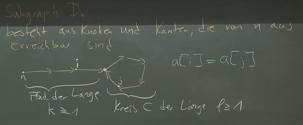
Phase 1 Prove that s.t. .
- let (as )
- then is on the cycle .
- is a multiple of
- thus
- as means we are already on the cycle, then advancing another steps (i.e. a multiple) of means we end up at the same place
We can also prove that now:
- as means we are already on the cycle, then advancing another steps (i.e. a multiple) of means we end up at the same place
- and as there are only nodes on the graph (and there can be at most n nodes)
Phase 2 Prove that for with .
- thus
- thus as we move times around the cycle when starting from (the beginning of the cycle).
# First phase
hase = a[n]; igel = a[a[n]]
t = 1
while (igel != hase)
	igel = a[igel]
	hase = a[a[hase]]
	t++

# Second phase
hase = n # reset to start
while (hase != igel)
	i = hase; j = igel;
	igel = a[igel]
	hase = a[hase]
return i, j
Runtime , as and . The total runtime is .
3.1 Graphenalgorithmen
3.1.1. Lange Pfade
Wir wollen für einen Graphen und feststellen, ob es einen Pfad der Länge in gibt. Wir nennen dies das LONG-PATH Problem.
NP-Reduction The problem is probably not solvable in polynomial time, as we can show that for it’s equivalent to the Hamilton-path problem (which is NP-complete).
We transform in the following way:
-
we choose any .
-
For each , we create a new node and insert the edge .
This results in with at most nodes (as ). -
(1) has Hamilton-path has path of length
- Let be a Hamiltonpath in
- Wlog let .
- Then is a path of length in
-
(2) has path of length has Hamilton-path
- Let be a path of length in
- Note that have to have
- thus they have to be exactly the surviving nodes after changing
- Thus and have exactly . Thus and
- Then is a Hamiltonpath in
We can thus transform in at most.
3.1
LONG-PATHreductionIf we can solve
LONG-PATHfor a graph with nodes in , then we can solve the Hamiltonpath problem in .
What about long-paths with ? we have indeed found a polynomial time algorithm for this: Color Coding
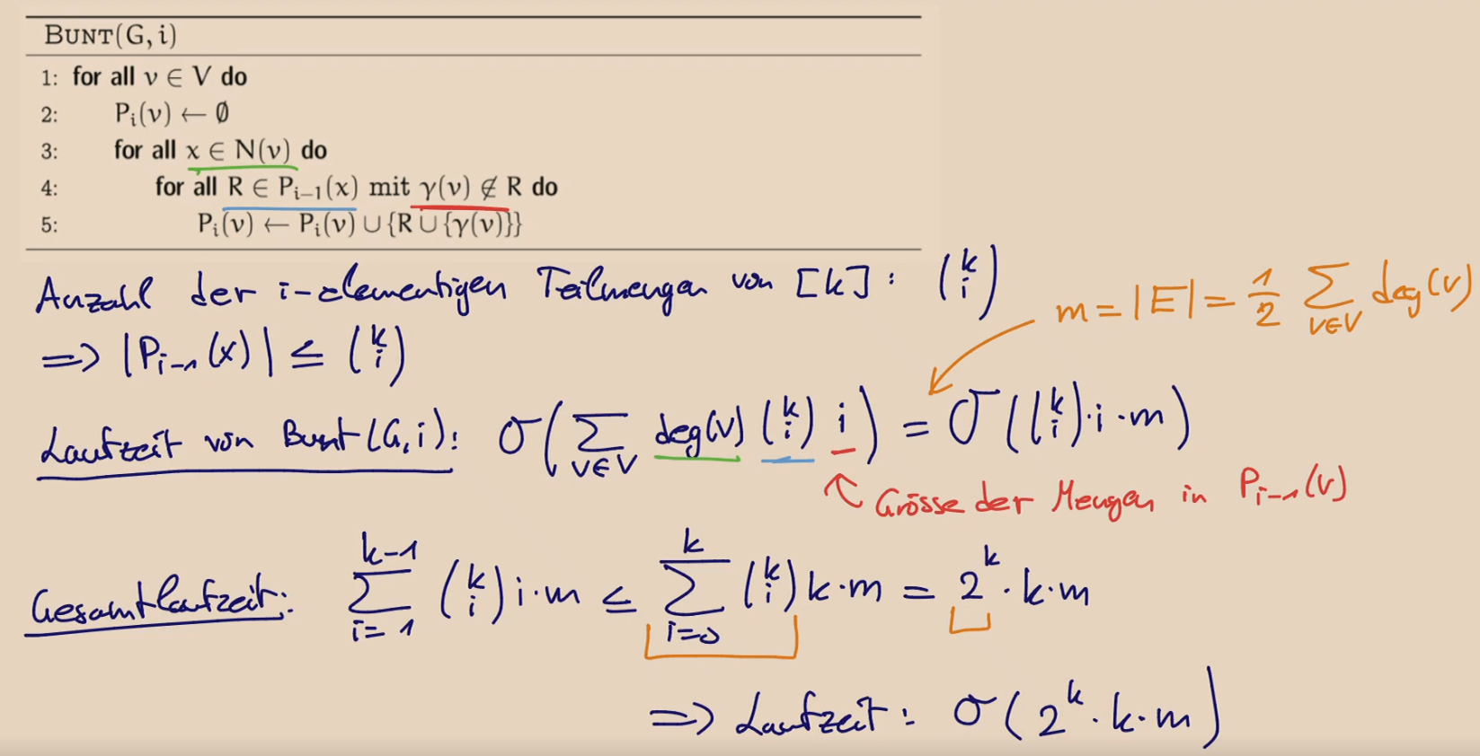
Bunte Pfade
Sei ein Graph mit einer Abbildung . Ein Pfad ist bunt, wenn alle Knoten verschiedene Farben haben.
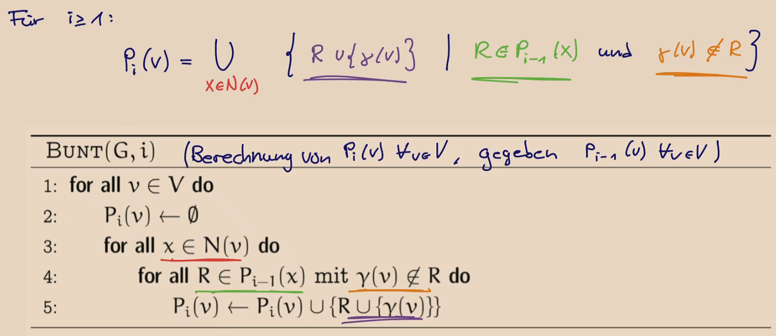
On the basis of this definition, we now define the following set for and :
The following is an example of :
-def.png)
contains a set of colours iff. there is a colourful path ending in , whose colours are exactly .
- Such a path must always have length .
- Every such path contains .
DP-Algorithm If we can calculate the set for all , our problem is solved as
Base Case:
Thus we can write our recursion step as
Runtime
Solving LONG-PATH We now can check if a path of length exists in a coloured graph. How do we colour it to get polynomial runtime?
- we randomly assign a colouring with colours, .
- if there is a colourful path of length , there is definitely a path of length
- if not, we might have had bad luck
Probability of finding a path if it exists Assume that contains a path of length .
- there are possible colourings
- in of these cases the path is colourful.
3.2
Let be a graph with a path of length
- A random colouring with colours creates a path of length with
- If we repeatedly randomly colour the graph and check, the expected number of times is
Proof (2) holds as and thus .
We can now easily construct a Monte-Carlo algorithm (as the runtime is constant - as we choose it, but the output is not always right), which solves the problem in polynomial runtime.
- We choose , and repeat our test times, until we get a
YES. If we never get one, we returnNO(but we are unsure, maybe we should have tried more).
3.3
- The algorithm runs in
- If the graph has a path of length , the probability that the algorithms outputs
NOis at most .
Proof (3)
- we know .
- The probability our algorithm says no it at most
Note: We can make this deterministic (i.e. non-random)
- there is a family of colourings
- For every subset of size , some colouring in gives all elements in different colours
These are called -perfect hash families.
— Aside → these are related to the universal hashing schemes used for hashmaps. (they are the existential, worst-case sibling)
Note: In acyclic graphs this problem becomes easy → we simply assign weight to each edge and search for shortest path. Then run over it with Bellman-Ford.
3.1.2 Flüsse in Netzwerken
Network
A network is a tuple where:
- is a directed Graph
- is the source
- is the sink
- de capacity function
The capacity of an edge limits the amount of “water” or anything really that flows through it.
There is another constraint: the network is closed, similar to Kirchhoff’s law for electronics. The sum of inputs / outputs at each node is 0 (except source and sink).
3.5 Zulässigkeit & Erhaltung
Let be a network. A flow (Fluss) in is a function with the constraints:
- for each (except )
- For all :
(incoming = outgoing of a node)
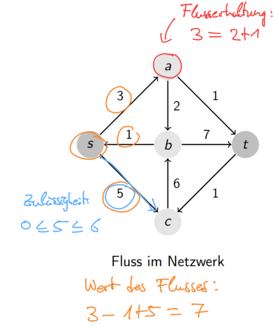
3.5b Value of a flow
The value (Wert) of a flow is defined as
Note: is not . → This means that a source can have incoming edges of non-zero capacity as well!
- the source/sink here are not the strict definitions from before (no incoming / outgoing edges)
Note: a flow can have a negative value (more incoming than outcoming - ex: one edge with the flow could then have that edge with positive and we have negative value).
A flow is of integral (ganzzahlig) if , .
In our model, the value of a flow measures how much “water” is actually moved. Thus all that is going in also comes out → inflow = outflow.
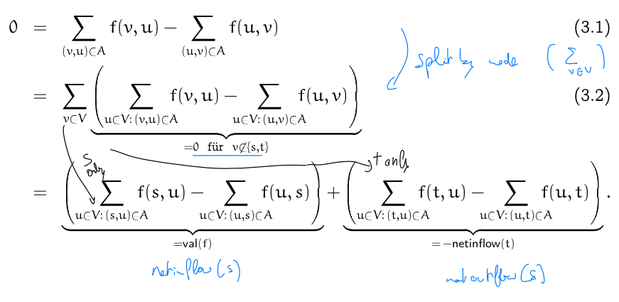
3.6 Nettozufluss
The net-inflow of a sink is equal to the value of the flow:
Proof
The problem we are interested in now is how to determine the “maximum flow”.
Note: it’s not clear such a flow always exists. For real capacities, it might be like having no largest number in it.
→ The way to solve this problem is to switch perspective and look at cuts (specifically minimum cuts)
3.7 --Cut
An --cut for a network is a partition of with and .
The capacity of a cut is given by
i.e. the sum of all edges crossing the cut from (note: those in the reverse direction are not subtracted).
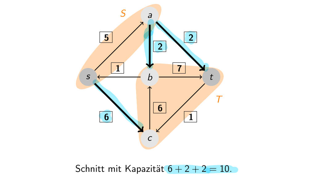
3.8 Cut Flow
Is a flow and a cut then
Proof: For a partition of
We want to prove
note, for (ii) we are basically only using that . For (iii) we are just using .
All cuts have same flow (CLRS p.721)
Shown in (i): For a flow , no matter which cut we choose, the net flow crossing that cut is the same and equal to the value of the flow.
i.e. for all cuts.
- (i) → similar structure to before
- (1): is just the definition
- (1) $\to$ (2): since by Flusserhaltung, for $v \neq s$ $\sum f(v, u) - \sum f(u, v) = 0$, we can rewrite the sum over all nodes in $S$
	- note this is not true for $t$, but $t \not \in S$ by definition of the cut
	- all terms except the $f(s, u)$ and $f(u, s)$ sums cancel out.
- (2) $\to$ (3):
  we take the double sum and regroup it by if the edge crosses or does not cross the cut.	  ![[cut<=flow.png]]
   - (3) $\to$ (4): just definition as stated before
Details on (2) → (3): We can split the sum in the following way due to the observation that edges that cross the cut are not cancelled

As every network has only a finite amount of cuts ( of them to be exact) there is in all cases a minimum cut. With the next theorem, we show that finding the minimum-cut is the dual of finding the maximum flow.
3.9 Maxflow-Mincut Theorem
Every network satisfies
Note: the asymmetry of subtracting edges crossing the cut from the flow but not their capacity from the min-cut is important: otherwise you could have .
we already know from the lemma 3.8
→ we will prove the equality now, by construction using the Ford-Fulkerson algorithm. (i.e. we show such a maxflow exists)
We can find a maximum flow iteratively, by repeatedly increasing it along augmenting paths.
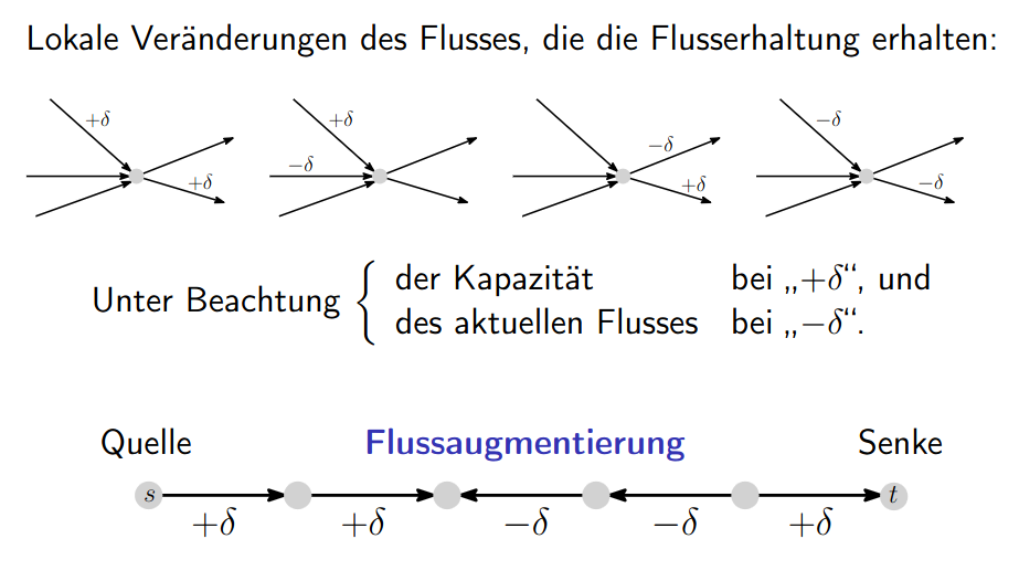
Note: we can increase the overall value of the flow by decreasing the flow along “backwards” edges (this allows us to push more through the forward ones).
Note: this only works in networks with rational capacities. If they were real we could not guarantee to reach the max-flow in a finite time.
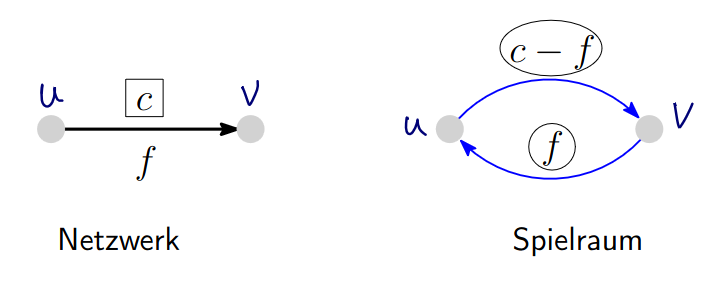
Restnetzwerk (Residual network)
Let be a network without multi-edges. Let be a flow in .
The residual network is defined as follows:
- if with , then there is also an edge in , with
- If with then there is in , with .
- Only edges like in (1) and (2) are in .
is called the rest-capacity of an edge in .
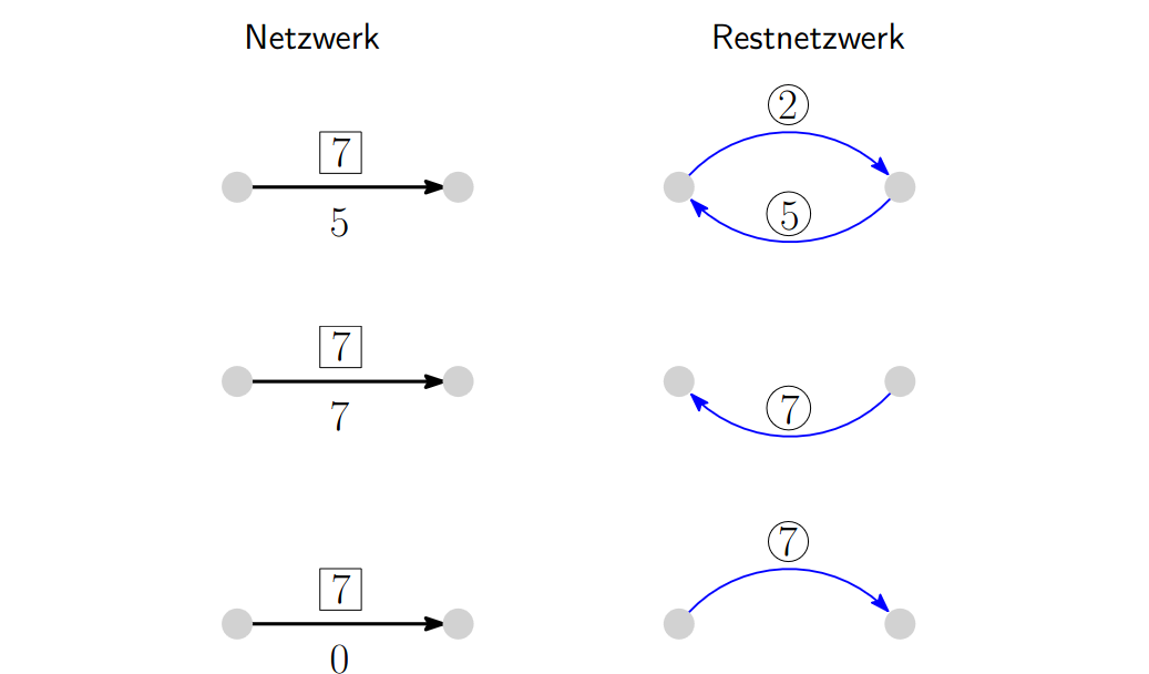
Note: for all and (since each edge becomes at most 2 new edges).
Some examples of edge-cases:
3.11 Maximal Flow in residual network
A flow in a network is a maximal flow iff. there is no directed path in the residual network from to .
For every such flow there is an --cut with .
WARNING! Exam Relevant: when executing the algorithm by hand, the will be all nodes reachable in the residual network, not !
Proof:
- assume there is an --path in . Let be the smallest residual capacity on this path (then , otherwise no path).
- then we can turn into by
 - by doing this $f'$ can not turn negative and always stays within capacity limits. We also respect flusserhaltung by adding / subtracting the same $\epsilon$ from each node.
 - Thus $\text{val}(f') = \text{val}(f) + \epsilon$ and $f$ could not have been maximal.
- Assume has no path from to .
- Let be the set of all edges reachable from directed edges in (note: in the residual network!).
- We know , (otherwise we’d have an augmenting path). Thus is an --cut.
- For with and , then there is no edge in
- thus otherwise there would be a residual edge and
- For with and , then there is no edge in
- thus otherwise there would be a residual edge and /.
- thus
- and by Lemma 3.8 .
- Thus is maximal (as it’s bounded by the capacity of all cuts).
- Let be the set of all edges reachable from directed edges in (note: in the residual network!).
The following algorithm now allows us to incrementally augment the flow and find the max-flow.
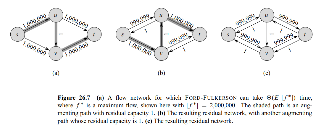
Note: Ford-Fulkerson as shows does not specify which --augmenting-path to choose. In the worst-case, we could be increasing only by each time. Edmonds-Karp solves this issue by using BFS to find the shortest (by edges) augmenting-path!
- Edmonds-Karp runs ins at most.
Example of a worst case for Ford-Fulkerson:
- DFS tricked to choose s → u → v → t, then s → v → u → t (if v, u before t in the ordering)
- BFS always finds the shortest paths → i.e. directly s → v → t or s → u → t.
Runtime of Ford-Fulkerson
If the capacities in a network without opposing edges are integral and at most then there is an integral maxflow that can be found in .
It’s clear that the smaller the better the algorithm (often we can get away with for special cases - matching, etc…).
As long as the capacities are integral, we can augment by at least if the flow is not maximal → this guarantees it terminates.
We have now proven maxflow-mincut.
Analysis
- worst case. Thus there are at most augmentations
- Each augmenting path can be found in time.
Extra:
- using capacity-scaling we can show that there is an algorithm finding the maxflow in time .
- using dynamic trees we can show the flow can be found in time at most.
3.1.2.2 Bipartite Matching as a Flow Problem
(CLRS p. 732)
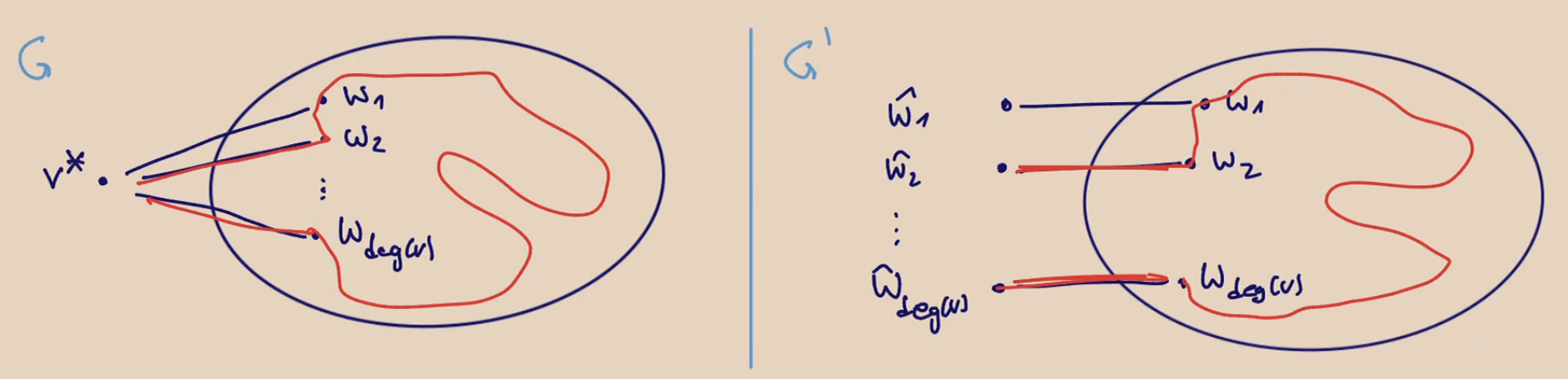
We can reduce the maximum bipartite matching problem onto a max-flow problem and use Ford-Fulkerson to find it.
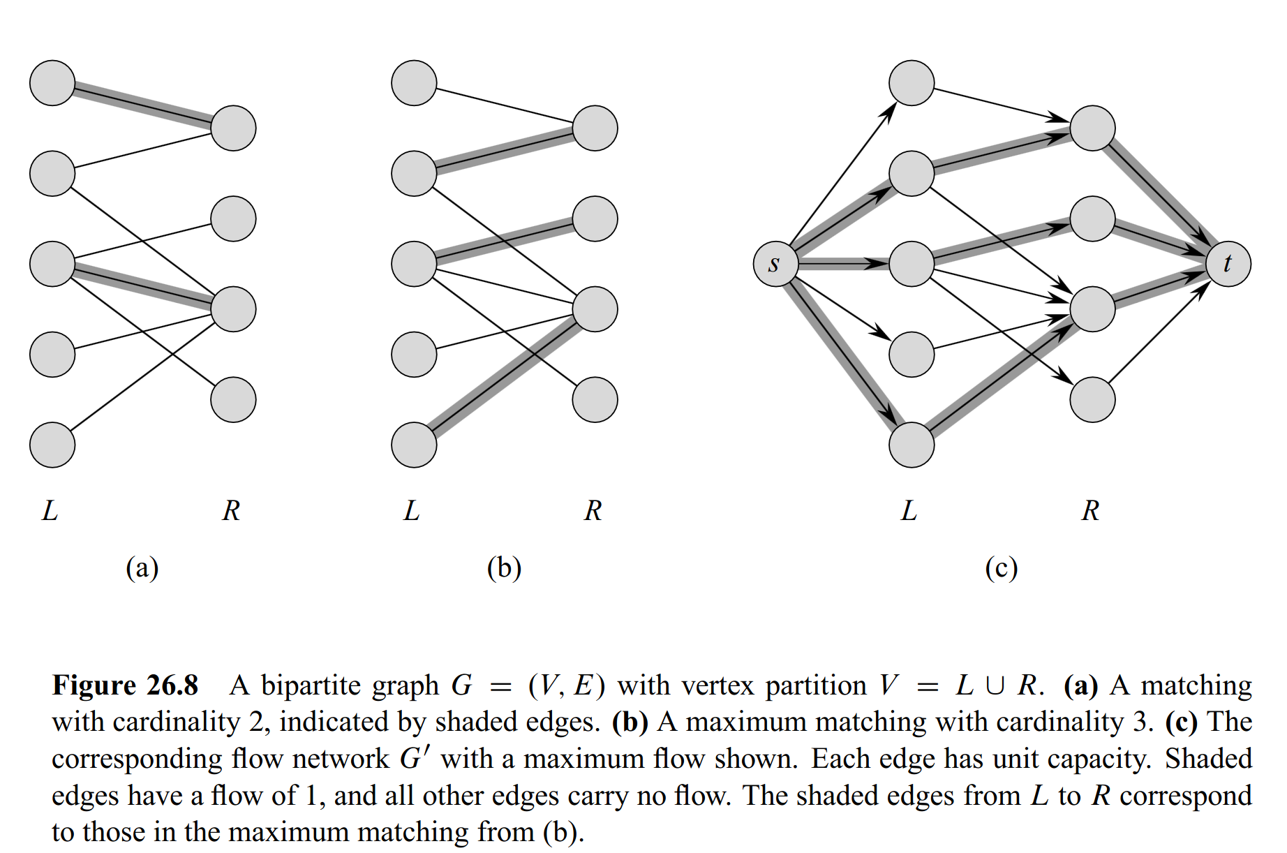
Each node in has only incoming edge of capacity , so only one outgoing edge with can leave at most. Every node in has only one outgoing, so only incoming edge with can exist. Thus every flow is a valid matching.
Since Ford-Fulkerson has only integral-capacity flows, an edge can either have . Thus a max-flow produced by FF is always a valid maximal matching.
3.15 Matching as max-flow
The size of a maximal matching in a bipartite Graph is equal to the value of a maximal flow in .
Note: we can use this to prove 1.6.2 Der Satz von Hall for example.
3.1.2.3 Knoten- und kantendisjunkte Pfade
We can also model finding edge-disjoint paths in a graph as a maxflow problem.
First, we transform out graph into a network. Each undirected edge is modelled as two directed edges with capacity . The source and sink both have capacity and have only one edge into and respectively.
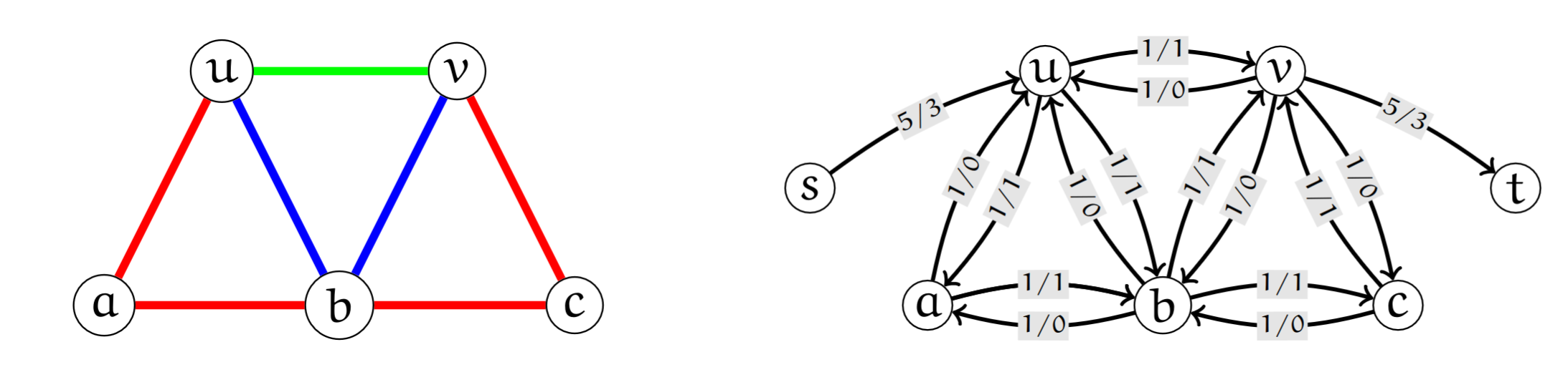
The max-flow in this graph is then equal to the number of edge-disjoint paths between and . This can be used to prove Menger’s Theorem.
How can we be sure every edge is only used once? Because if and , we can simply set both to , as they cancel out. This results in a flow with equivalent value (since no edge out of or into source/sink has been affected).
We can also do the same for internally node-disjoint paths: we split each node into and where there is only a single edge between . Thus we can easily see each node can only be used once.
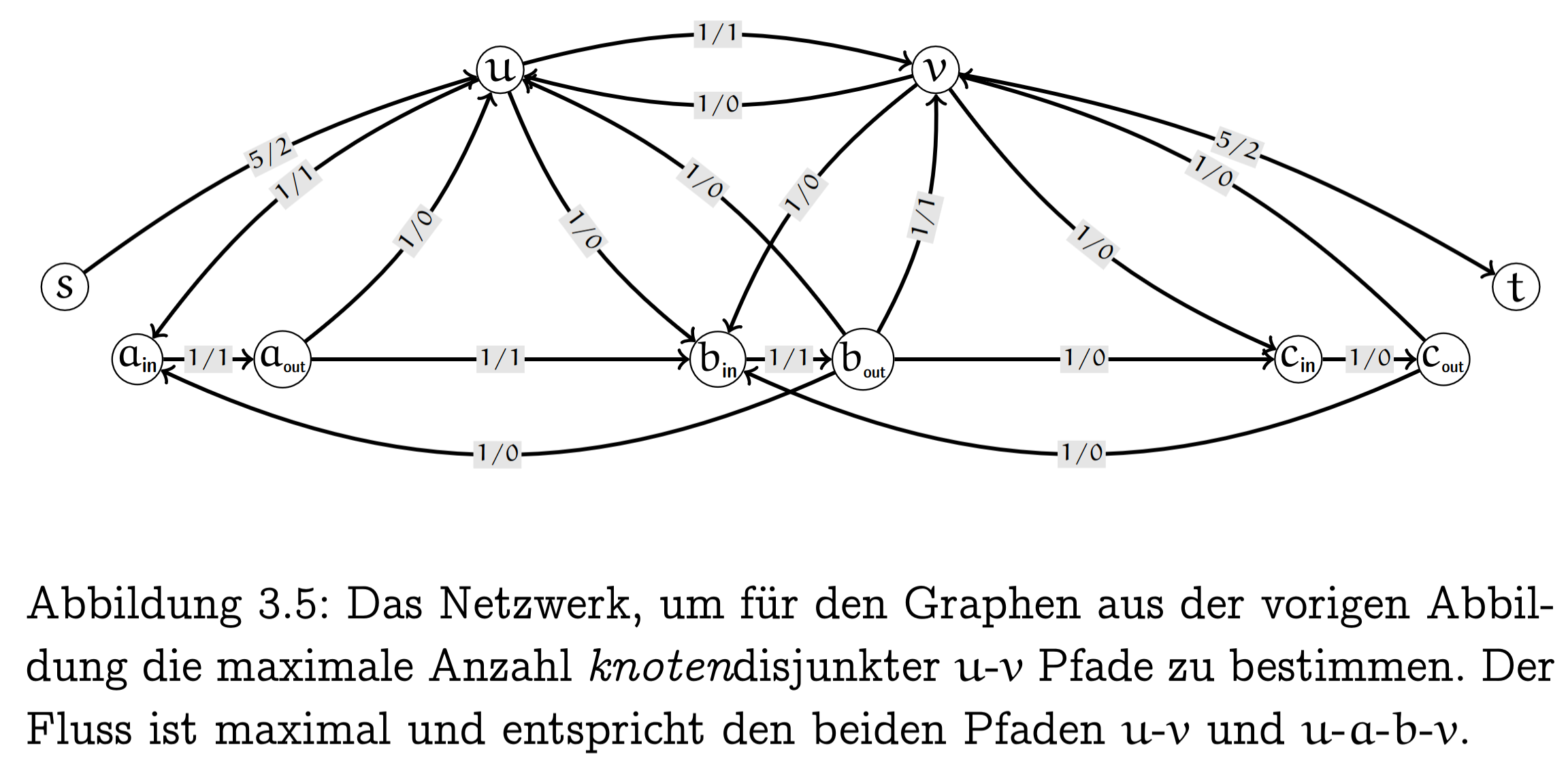
In general to make sure a node is used only once we can split it in two with a capacity 1 edge between them. Then all incoming edges go into the first and all outgoing leave the second.
3.1.2.4 Bildsegmentierung
We can also use flows to find a min-cut, corresponding to the best fitting “image segmentation” by some criteria → foreground / background separation.
We model the problem as for all pixel and for all of them as well. Each pixel is then connected to their cardinal neighbours via bi-directional edges as well.
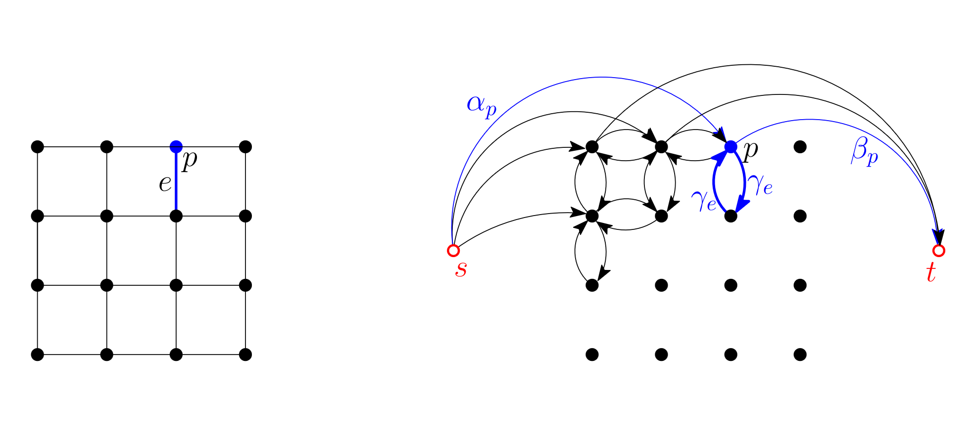
We obtain some for each pixel.
- Alpha is the “foreground-ness”
- beta the “background-ness”
- is defined for each direction as the “probability the neighbour is also foreground/background” → influence factor.
We then define the quality of our segmentation as follows:
it’s the sum of all terms that tell us how “correct” each pixel’s classification is. We subtract for each (i.e. “wrong edges”).
But we don’t know how to maximise this value → so we redefine and get a cut-minimisation problem: let
and minimising is the same as maximising .
We can see that the minimum cut minimises the quality function as well. We thus can apply a max-flow algorithm to our network and get the best segmentation.
3.1.2.5 Konvexe Mengen
Go to 3.2.2 Konvexe Hülle to read the definitions.
We can represent any network as , for any enumeration of all edges. Then each flow can be represented as a vector in .
The set of all flows can be seen as a subset of .
3.19
The set of all flows of network with edges is a convex subset of .
The set of all maximal flows is also a convex subset of .
Note: every problem modellable as having something to do with convexity is usually solvable fast (finding global minima is easy) → same as for training neural nets.
On the other hand, finding global maxima on convex plane is NP-hard.
3.1.4 Minimale Schnitte
The MIN-CUT Problem asks for the smallest cut that makes a connected graph disconnected. We denote the size of the min-cut on this graph.
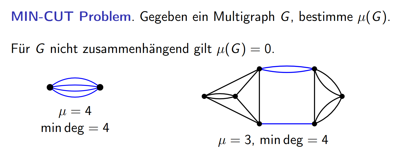
Note that the graph is a multigraph → to use existing flow modelling, we turn any parallel edges into an edge with # of parallel edges.
We can use the maxflow-mincut theorem to find a min-cut between and in . If we want to find the min-cut over an entire graph, we can simply repeat the algorithm times for any pair of vertices and get the min-cut.
As this gives a total of runtime.
We can do better by observing that we only need to fix a source and check all for total runtime.
- we only need to fix the source as there is no partition of such that all are on one side (i.e. a cut we haven’t checked) without .
We can do better however, by using a probabilistic method that utilises edge contraction.
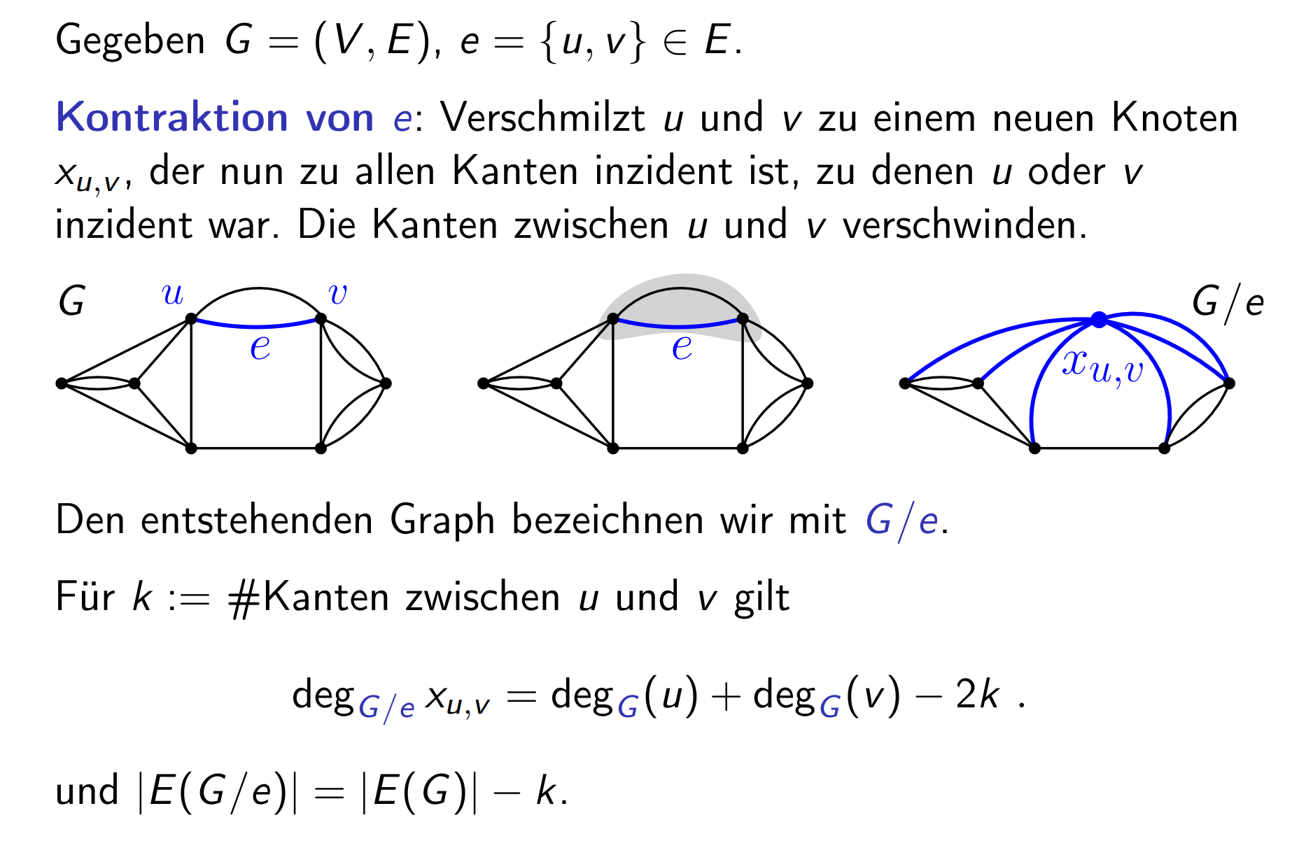
Now notice that this reduces the number of cuts that exist in the graph, i.e. it removes the cuts that contain the contracted edge .
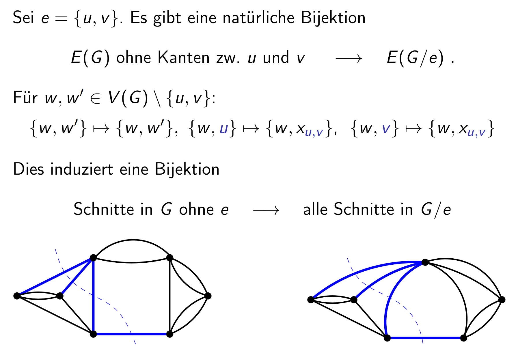
Let be a min-cut, i.e. . This bijection means that if we contract , .
3.20 Contraction preserves cuts
Let be a graph and an edge. Then
holds for all .
If there is a min-cut s.t. , then .
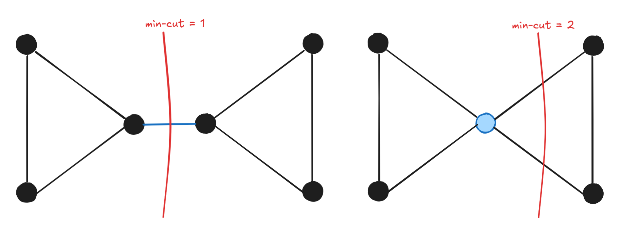
Note that this holds since any cuts with are preserved (subset). And doesn’t get new cuts (as it has less edges). Thus and thus the min can only be bigger in .
Just choose any : A priori there is no fast way of choosing an without knowing , so we’ll just choose a random edge.
We suppose we can contract and choose a random edge both in . Then CUT(G) can be implemented in .
The output will never be smaller as . As long as we’re lucky, we get . But how lucky?
3.21 Probability of success
Let , . For chosen randomly we have
Proof:
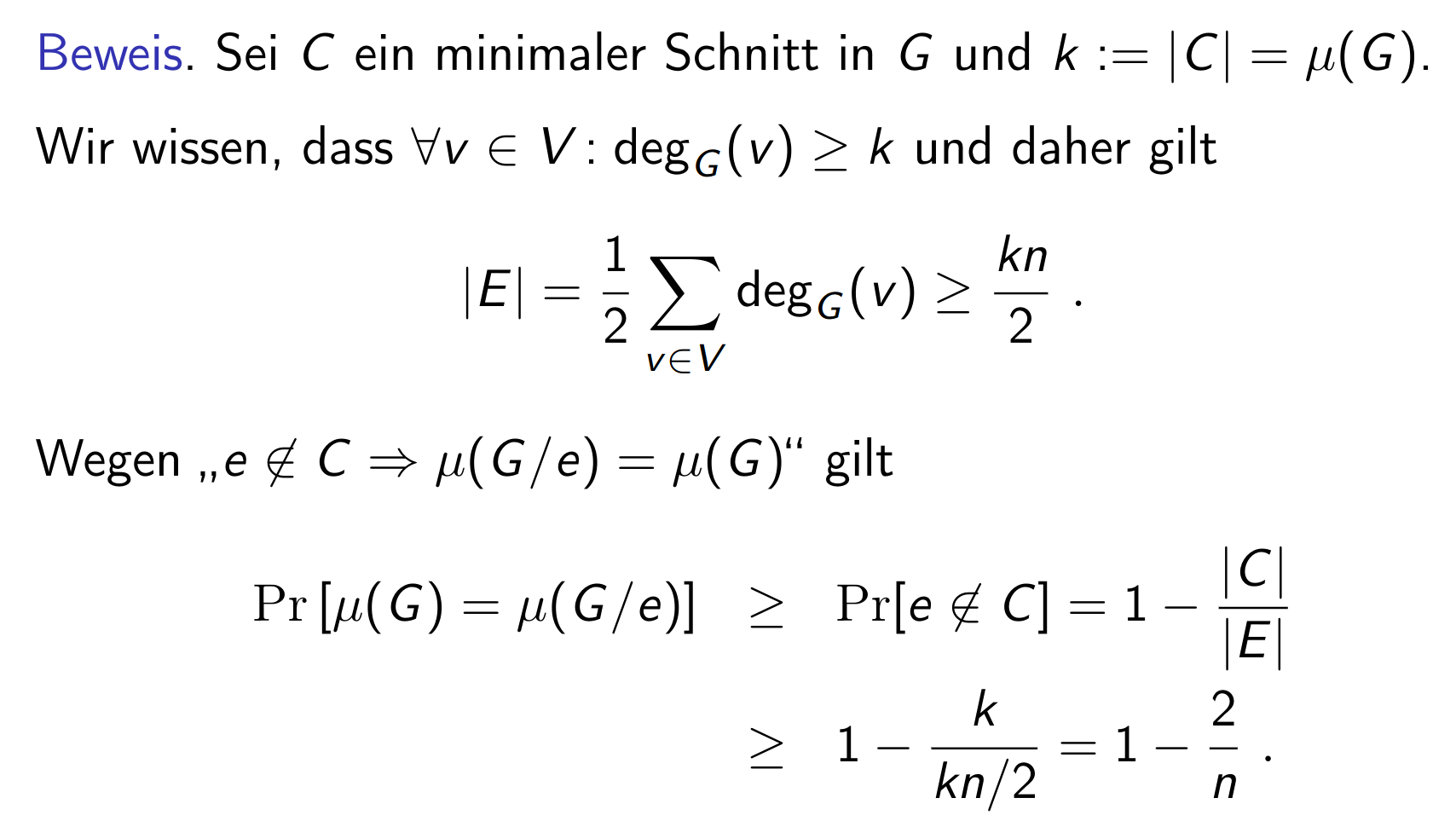
Note that as is fixed. There might be another min-cut which does not contain and does not in fact increase. Thus bigger equals.
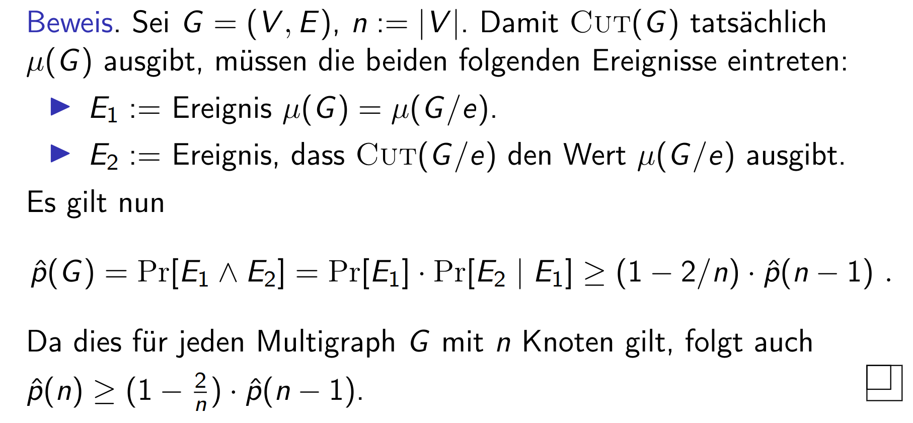
Now probability over entire execution:
Let probability that CUT(G) outputs . And let (infimum instead of minimum because there is an infinite amount of multigraphs of size ).
3.22
Proof:
If we recursively insert the definition, this gives us a telescoping sum:
3.23
Es gilt
Thus CUT(G) is a Monte-Carlo algorithm with probability of success .
3.24 Repeat
We repeat the algorithm times.
- runtime
- probability of success .
We choose . Then
using familiar rules. And because we get the above value.
Now for we get probability of success and runtime . We already had this before, even without failure, so what did we gain???
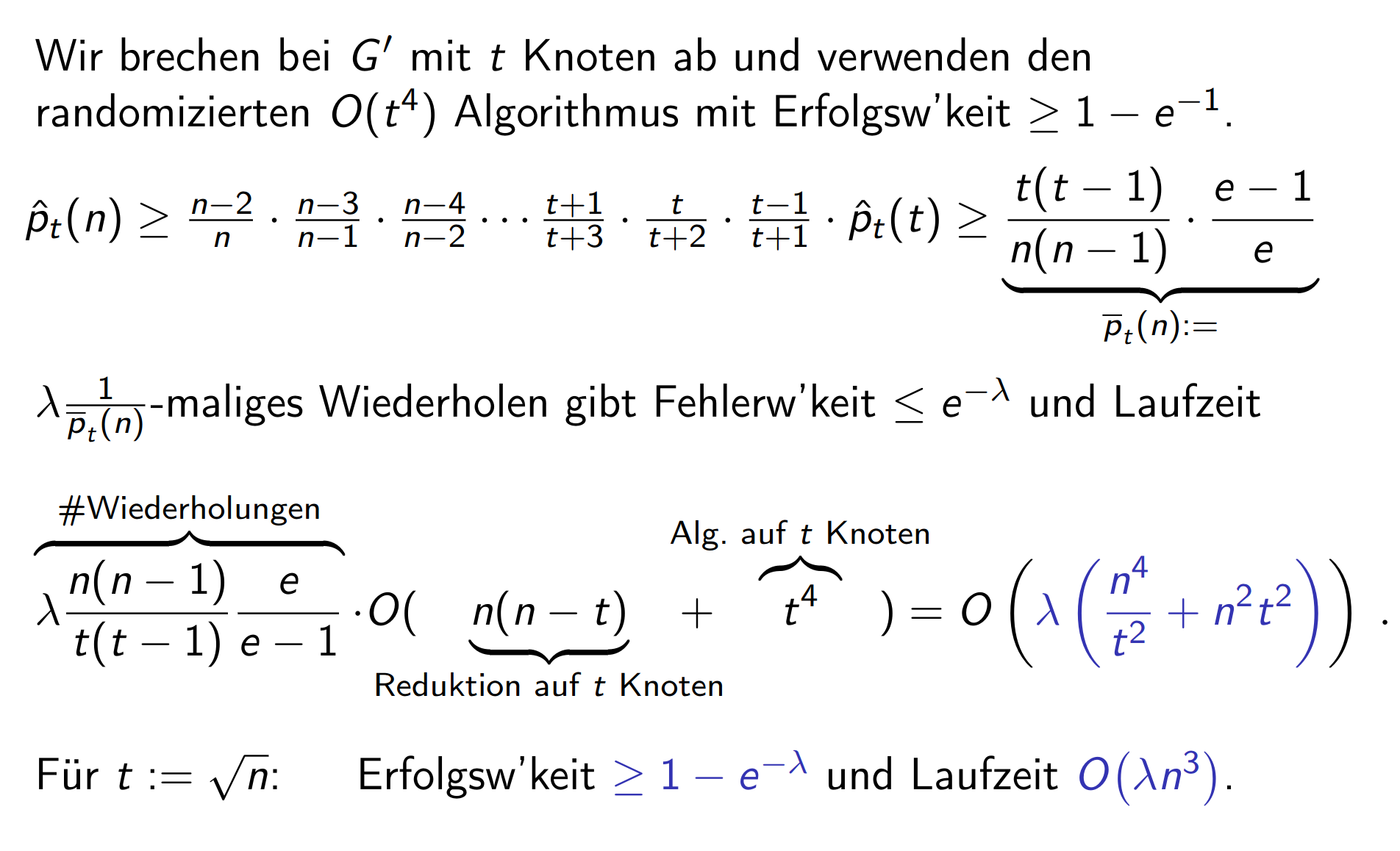
Bootstrapping: Because for small values of our algorithm is so bad (for we have chance picking the right edge), we can consider cutting off early at and continue using our deterministic algorithm.
Or we choose to put our own probabilistic algo into itself, and reuse it internally with repetitions.
- how is this different than just continuing? instead of picking an edge at random, we run
CUT(G'), so for all possible pairs of contractions left. - and so we expect to get the actual min-cut for the graph of size back.
Then we get runtime for the same expected error probability:
Now we can generalise this result. For an algorithm with runtime we already have, we can insert it and get one with runtime :
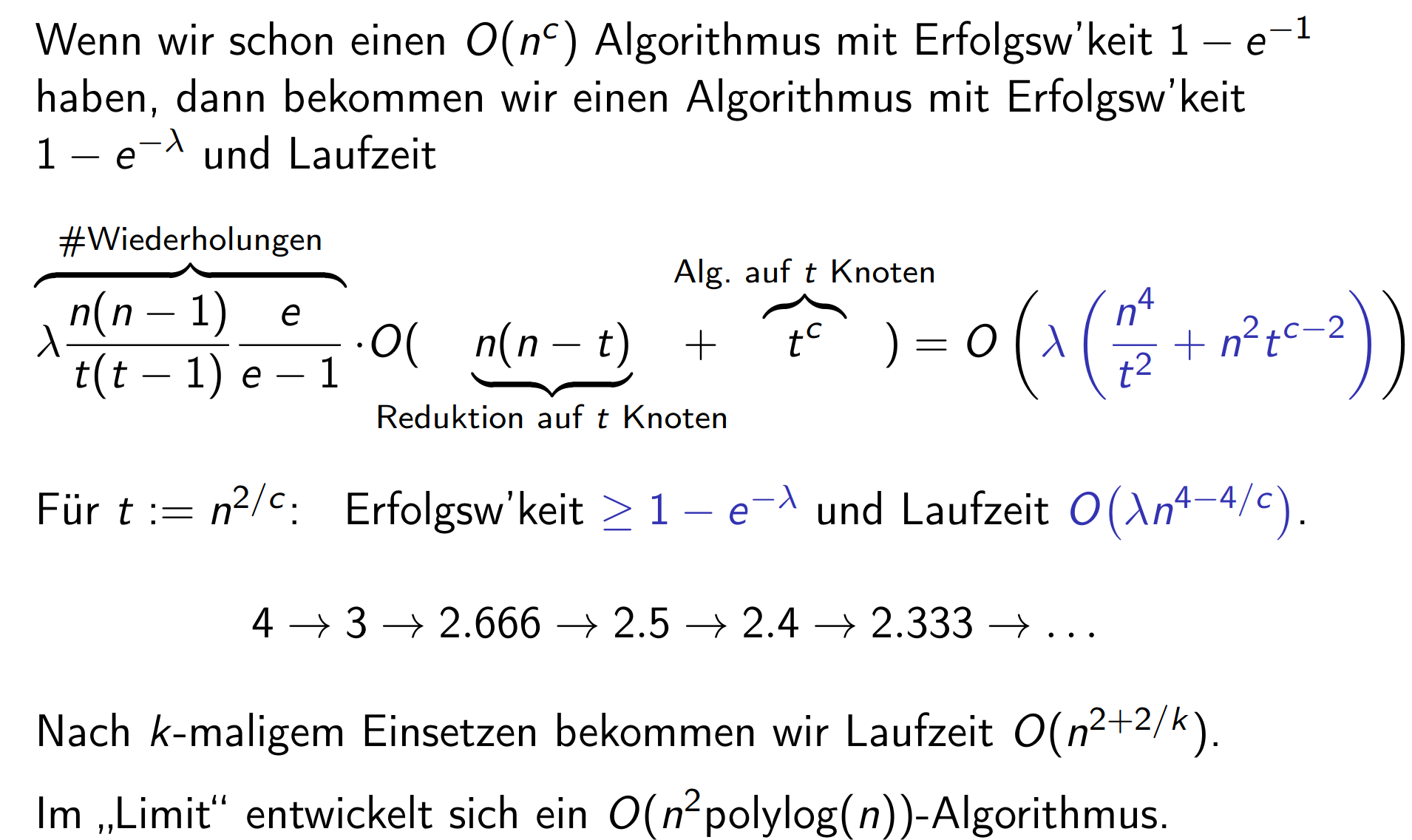
Finally, using this reduction process, we can derive an explicit formula for insertions: .
3.2 Geometrische Algorithmen
3.2.1 Kleinster umschließender Kreis
We want to find the smallest circle such that all points are inside it. (We will assume the proof of existence for such a circle.)
3.25 Uniqueness
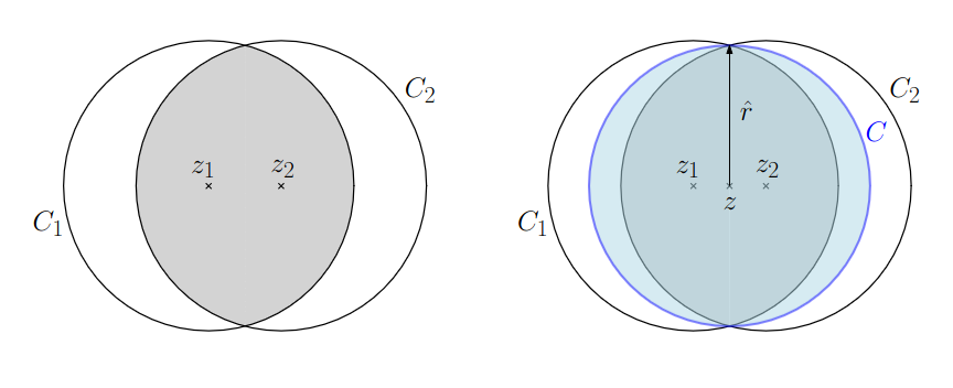
For every finite set of points in there is a unique (eindeutig) smallest enclosing circle .
Assume there are two WLOG such that and . Thus . We can then create a new smaller circle from the midpoint of both centers.
3.26 3 Points suffice
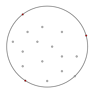
For every finite set of points with there is a subset s.t. and .
This follows from the fact that there is no arc through the middle for which all points are on one side only.
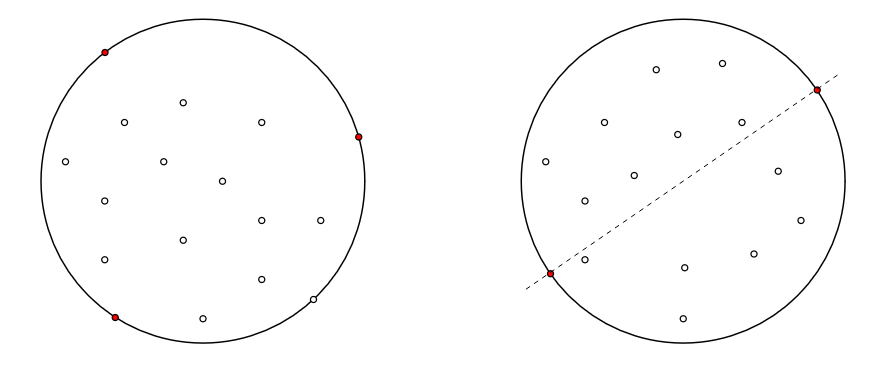
If there was, we could create a new smaller enclosing circle → contradiction:
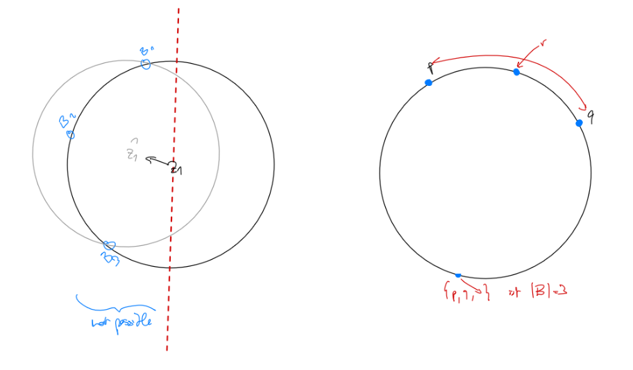
Let be the set of points on the circle. If there’s two points exactly opposed, we can just take any random third. If there’s more than , take and then any except the points in the smaller of the two arcs (as illustrated above).
Algorithm 1: From this we can immediately derive an algorithm.
We iterate through all subsets of size $3$ in $O(n^3)$ and check for enclosing in $O(n)$. Note that this works since $C(Q) \le C(P)$ since $Q \subseteq P$!Note: We can make this by instead iterating over all and taking the largest. This works because there s.t. always exists.
Algorithm 2 (randomised) We can also randomise this.
This is still $O(n^4)$ since worst case there is exactly one unique $|Q| = 3$. Then we need to iterate over *all* subsets of size $3$ of $P$. The $\E[\text{draw } Q] = \binom{n}{3}$ as it's geometrically distributed with $p = 1/\binom{n}{3}$.First idea: maybe we could draw more than only points? This does not change the runtime of the algorithm in the worst-case however.
Algorithm 3 (randomised) Instead, we increase the chance of points outside being drawn.
- Las Vegas
- runtime is ZV as we have to be lucky to draw the right set of points
- but we can easily verify if correct (check all points) → always right answer
3.28
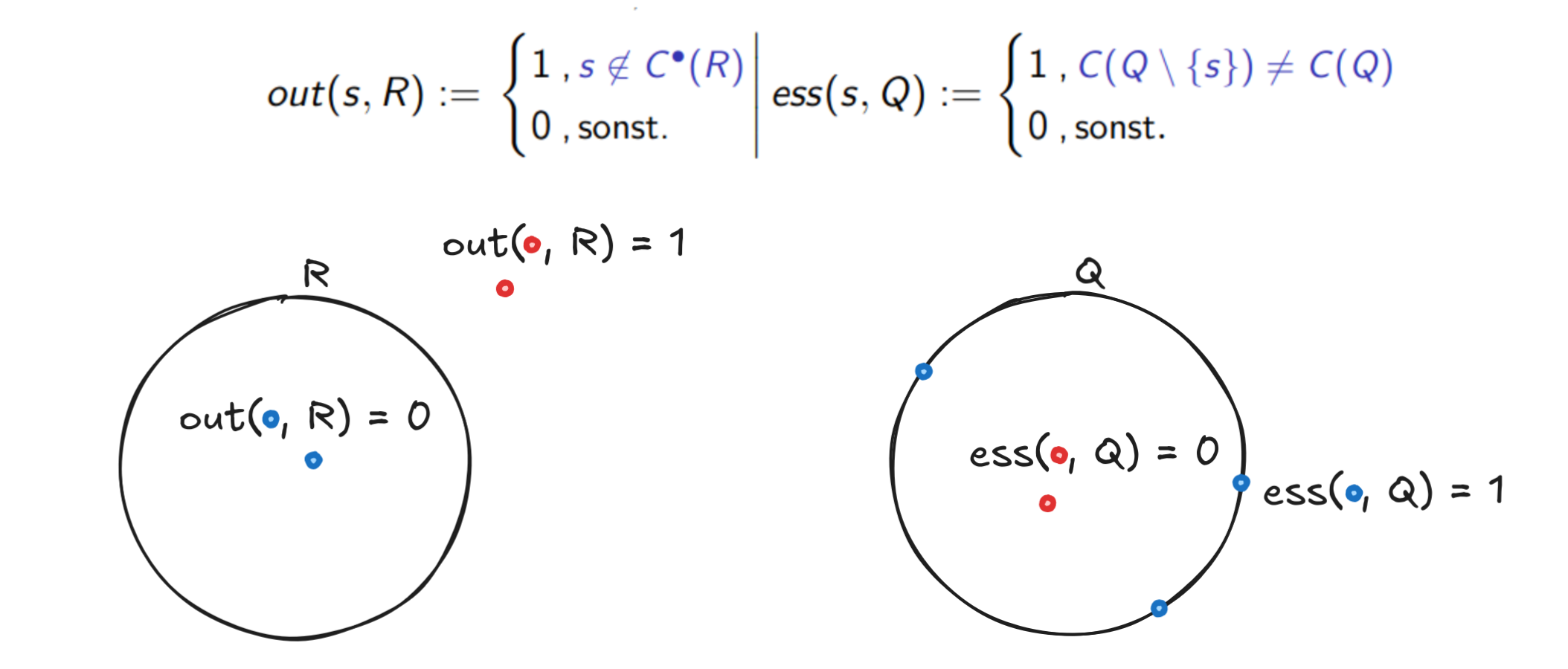
Let be a set of (not necessarily different) points and for uniformly chosen from . Then the expected number of points in that are outside of is at most
Proof: We define two helper functions
- which is if
- which is if .
We can easily see that (if it’s outside, it makes the circle bigger).
We also have (let be the set of points, including duplicates)
and
(as we have seen we only need points to define a circle at most).
Then let be a ZV counting the number of points outside the circle
(*) follows from the fact that trying all points outside is the same as including one more in and then picking one inside.
(**) follows from our Lemma that there are at most essential points.
Why do we need this? We can now calculate the number of points that are expected to be doubled each iteration.
3.29
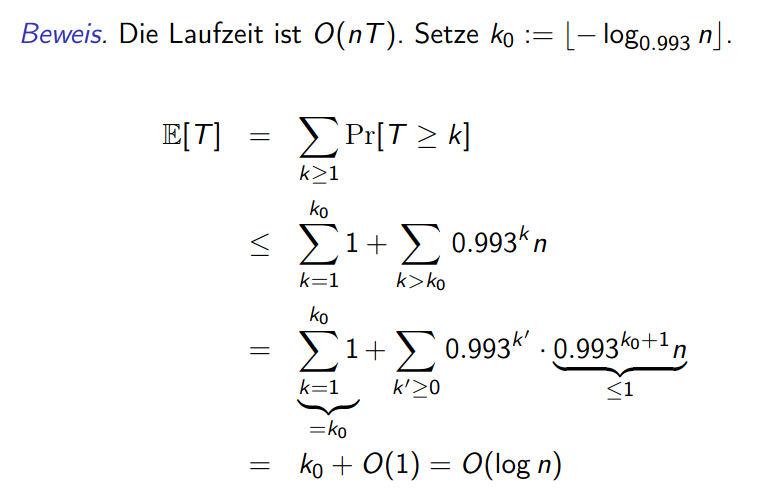
This algorithm calculates the smallest enclosing circle in expected time .
Proof Each round takes . How many rounds? (This is the sampling Lemma)
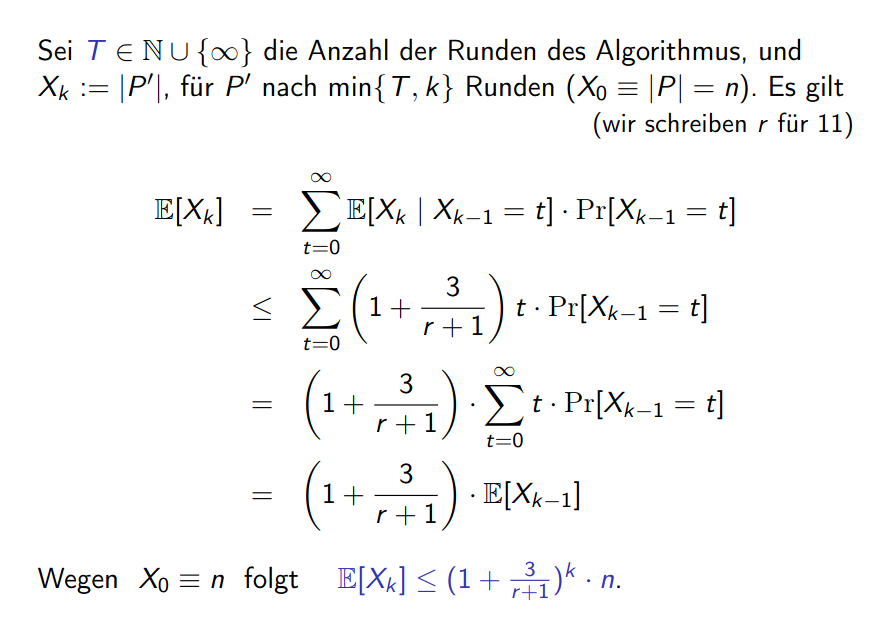
Note means that there are still rounds left to do. Thus , as at least one of the points in must have been doubled.
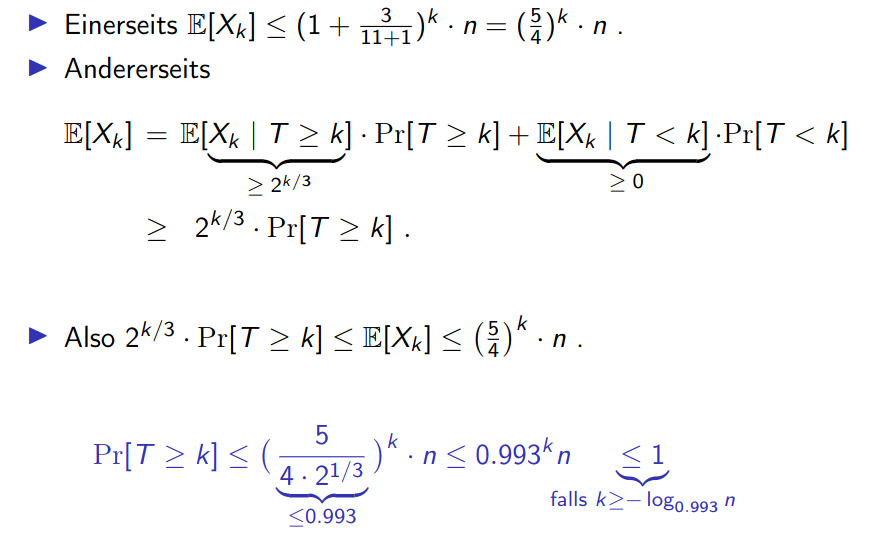
Note: we ignore the second term in and simply put lower bound in there.
Now we can estimate the number of repetitions:
(Aside) Sampling Lemma
We can make the observations from the previous algorithm more abstract.
For any problem statement with a set and a function (where is subsets of ), we can define:
which are the abstract equivalents of “out” and “essential” from before.
3.31 Sampling Lemma
Let , . Let and with a -element subset of , uniformly chosen.
Then for
From which we can derive the conclusion we came to for the smallest enclosing circle (chose , ).
Proof: this can be proven using a bipartite graph with edges for if (i.e. verletzt ).
- thus the degree of node is and there are exactly edges in the graph
- using the equivalence “out” ⇐> “ess” we proved before, we can switch to seeing the edges as and extreme in , i.e.
- then the degree of each node is exactly .
- the number of edges is .
Therefore → we can derive the lemma equality from this.
3.2.2 Konvexe Hülle
The convex hull problem is similar to the problem of the smallest enclosing circle, but only with a polygon instead of a circle.
3.33 Convex Hull
Let , . The convex hull of is the intersection of all convex sets containing :
Note: we can alternatively define it as:
- the cut of all “half-planes” (halbebene), die enthalten
- the smallest convex set that contains
A few definitions from the flow section again:
Line segment
For let
be the connecting line segment.
Convex set
A set is called convex if
The ConvexHull problem asks to find the smallest enclosing polygon conv(P) for a finite set of points . The output will be a set of points in counterclockwise order.
For our problem, we’ll assume a few simplifications for easier proofs:
- finite set of points .
- is in “allgemeiner Lage” so no 3 points aligned and no 2 points share an coordinate.
we’ll discuss how to get rid of them later.
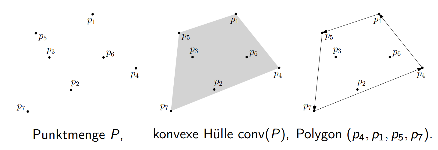
A key notion is the Randkante (boundary edge):
- an ordered pair with , , is a boundary edge of if all points of lie left of
- i.e. on the left side of the directed line through and , oriented from to .
3.34 Boundary-Edge Characterization
is the counterclockwise corner sequence of the polygon enclosing if and only if all pairs , , are boundary edges of .
The geometric primitive “is left or right of ?” is answered by a determinant.
3.35 Orientation Test
Let , , in . Then and lies left of if and only if
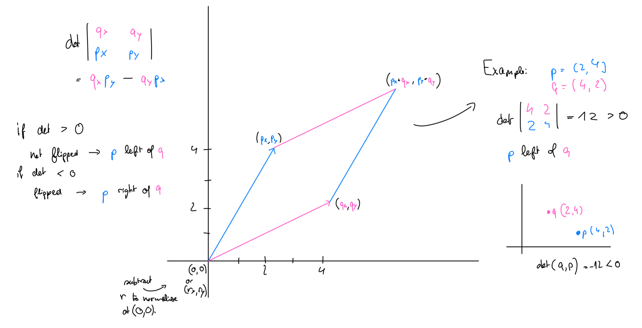
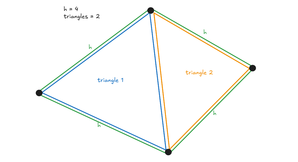
More precisely, is the area of the triangle :
- this happens counterclockwise (the positive, “normal” orientation in mathematics) and is left of .
- if , it’s flipped.
- the three points are collinear — which includes the degenerate cases where two of them, or all three, coincide.
First naive Algorithm .
Iterate through all and check if it’s a Randkante by checking for all other points if they’re on the left.
This takes for finding all pairs and to check if all points are on the left.
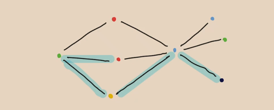
3.2.2.1 Jarvis’ Wrap
Second Approach (Jarvis’ Wrap): , number of Randkanten of the hull.
We can improve the brute-force approach by instead “wrapping” around the hull. We start with the lowest point (for sure a corner point) and find the next on the corner iteratively, until we’ve gone around.
point with smallest x-coord in (for sure part of the hull)
we start with :
Why does this work? The procedure mirrors finding the minimum of a set of numbers. Given , define a relation on by
3.36 FindNext Correctness
If is a corner of the convex hull of , then is a total order on . For the minimum of this order, is a boundary edge.

The essential property coming from ” is a corner of ” is that there exists a line separating from .
- If no such line exists, is cyclic → definitely not a total order
This gives us the following algorithm. Since we’re sure to start on a corner and only advance if we found another corner, we never get a degenerate case:
When running, this looks as follows:
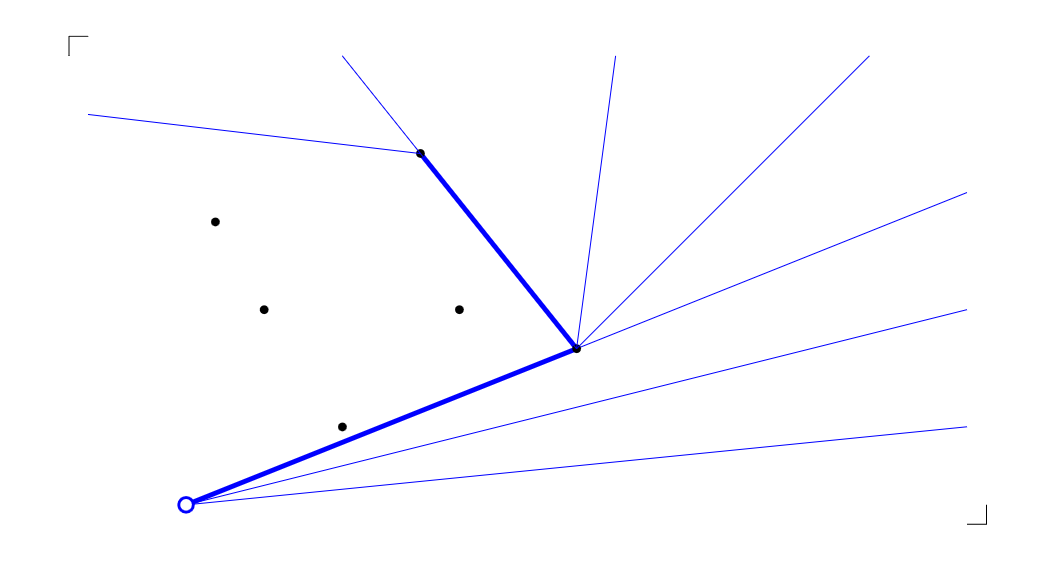
Each call to takes time, and we call it exactly times, once for each corner.
Jarvis' Wrap Running Time
Given a set of points in general position in , the algorithm computes the convex hull in time , where is the number of corners of the convex hull of .
This is very fast when is small (e.g. if the hull is a triangle the algorithm is linear), and in the worst case it still improves the first bound to .
What about without the initial simplifying assumptions?
- if there can be multiple points with same -coord, choose the one with smallest from them (lexicographic) to start on
- The test ” right of ” must be replaced by
- ” right of ” OR ” on the line through and .
- if we get as an array with duplicates, we need to make sure to not check the same point against itself.
If we implement this on a computer using floating point, we might run into some issues:
- accidentally make a slightly smaller hull, because of imprecisions
- we might run around the “starting point” because of imprecisions or because the starting point exists multiple times and never terminate
3.2.2.2 Local Improvements
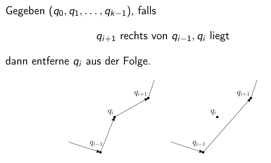
Begin with a polygon with corners from and successively “correct” it whenever we spot a “concavity”.
- If sequence bounds a convex set counterclockwise:
- must lie right of for all
- Whenever lies left of , we remove from the sequence, repeating until no such defect remains “Verbesserungsschritt”
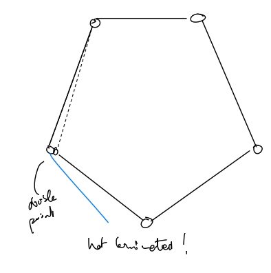
Note: the absence of a defect does not guarantee we have found the correct polygon → see this example of a locally convex polygon that is not a hull.
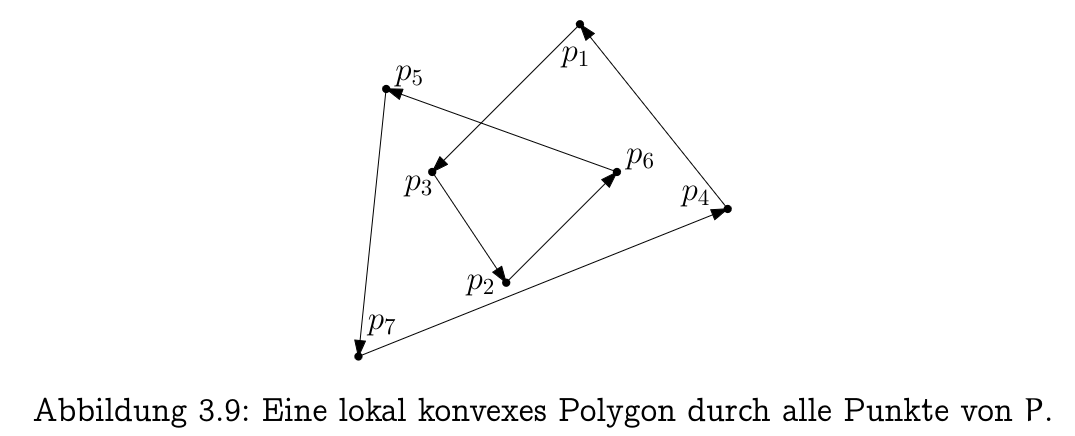
- do not even know if the polygon encloses
- even if every point of appears in the sequence → might have a closed, locally convex polygonal chain that self-intersects (see above)
Improvement Step ( Verbesserungsschritt)
An improvement step is the operation in which, for three consecutive points , we find that lies left of and therefore remove from the sequence.
In practice, this looks like the following:
Algorithm Idea:
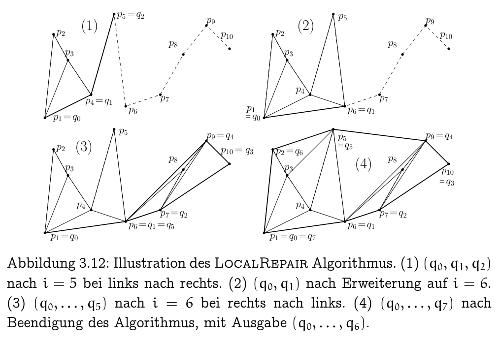
First sort ascending by -coordinate; let be the resulting order. Consider the polygon $(p_1, p_2, \ldots, p_{n-1}, p_n, p_{n-1}, \ldots, p_2):

We walk through once left to right and then back right to left.
- polygon has directed edges.
- Local repair never removes or
- at every moment the sequence splits into
- an -monotone part running from to (x increasing)
- second part running from back to
Note: If we keep the old edges in the drawing, we obtain at the end a Triangulierung (triangulation) of the point set .
We start with a polygon with corners → finish with corners.
- Each successful test ” and left of ” creates new triangle
- we know there are exactly of these
- there is exactly one unsuccessful test per new , in the lower hull and per new , in the upper hull
- giving an extra tests.
In total tests → !
- giving an extra tests.
LocalRepair Running Time
Given a sequence of points in general position in , sorted by -coordinate, the algorithm computes the convex hull of in time .
Including sort → algorithm = asymptotically faster than unless .
It is also relatively easy to handle points of equal -coordinate (sort lexicographically) and collinearities (repetitions can be removed after sorting)
- And Numerical inaccuracies cannot cause an infinite loop.
Can we do better? A sorting lower bound
We can reduce sorting onto the convex hull problem. Given a sequence of reals, set for .
- embed the on the -axis in and project them vertically onto the unit parabola .
Computing the convex hull of in our sense (sorted sequence of hull corners) yields (in linear time) the ascending order of the .
Thus: if convex hull can be computed in , then sorting can be done in time → contradiction with known lower bound of for sorting.
3.2.2.3 Triangulation (Extra)
3.38 Plane Graph
A graph on is called eben (plane) if the segments of the edges intersect at most in their common endpoints.
3.38 Gebiete
Removing the segments , , from yields connected regions, the Gebiete (regions) of . The bounded regions are the inner regions; the unbounded (infinite) region is the outer region.
3.38 Triangulation
A graph on is a triangulation of if is plane and maximal with this property,
Note: maximal means any edge from to violates planarity.
The regions of a plane graph on are all bounded except exactly one (the outer region).
- The inner regions of a triangulation are all triangles
- This is because any other polygon could be subdivided further
- the single outer region is the complement of in and borders precisely the boundary edges of .
3.39 Triangulation Counts from Local Repair
Let be the number of corners of the convex hull of . The local repair process makes exactly improvement steps and produces a triangulation with inner triangles and edges.
Proof:
- (i) Number of steps:
- We start with a polygon having directed edges.
- Each improvement step replaces two old directed edges by one new one, i.e. removes exactly one directed edge.
- Since we end with directed edges, we run exactly steps.
- We start with a polygon having directed edges.
- (ii) Number of triangles:
- We start with triangles, and each improvement step creates one new triangle. Over steps we obtain exactly triangles.
- (iii) Number of undirected edges:
- We start with undirected edges (counting each edge once, not twice for its two directions)
- add one edge per step, so we end with edges.
- (iii) Edge count, alternatively:
- Each of the triangles has three edges which each border two triangles (except for the boundary edges, so we add extra )
- Counting also the outer region with its edges, every edge is counted exactly twice. Hence the number of edges is
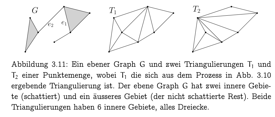
The Euler relation lets us extend these counts to all triangulations, not just those from local repair.
Euler Relation
Let be a plane graph on with vertices, edges, regions (including the outer region), and connected components. Then
Proof: we prove by “reverse induction”??
- The claim holds when : then there are connected components and exactly one region, so and , both equal to .
- Assume
- remove an edge , giving , which is again plane.
- Our goal is to show that the validity of (3.4) is unaffected by this operation:
Let be the values corresponding to for . We want to prove
Certainly and .
- What happens to and ?
- We do not choose arbitrarily:
- if possible, let lie on a cycle in ;
- if not, all connected components are trees and we choose incident to a degree- vertex (a leaf)
- → possible since , because every nonempty tree has at least two leaves.
Case 1: lies on a cycle in .
The number of connected components is unchanged, .
The cycle separates the two sides of , so borders two different regions of , which merge into one region in
Thus . Then (3.5) follows, since
Case 2: is incident to a degree- vertex in .
Then . The two sides of border the same region of , because we can travel from one side of the segment along and around to the other side without crossing any edge of
Thus . Then (3.5) follows easily.
By successively removing edges, (3.4) holds for if and only if it holds for the empty graph → which we already verified.
3.41 Edge and Region Counts for Plane Graphs
Let be a set of points in general position in , and let be the number of edges of .
- Every triangulation of has exactly edges and exactly inner regions.
- Every plane graph on has at most edges and at most inner regions.
Proof:
- (i) Let be the number of regions of . Then of them are inner regions (triangles), and the outer region borders edges. So the number of edges is . Since is connected, (3.4) gives
- so the number of inner regions is . The edge count then follows:
Moreover, and general position force .
- (ii) The bounds for follow because triangulations are maximal plane graphs
- adding edges to a plane graph only increases the edge count
- also never decreases the number of regions
Thus triangulations are sparse, with edges.
These definitions generalise in graph theory: a graph is planar if it can be drawn in the plane (edges realised as curves joining their endpoints) so that no two edges cross.