2. Entropy, Relative Entropy and Mutual Information

2.1 Entropy

Entropy

The entropy $H(X)$ of a discrete RV $X$ is defined by

$$H(X)=-\sum _{x\in \mathcal{X}}p(x)\log p(x)$$

Note: the log is in base $2$ as we express entropy in bits (changing the base of entropy just rescales it by a constant factor)

• we use the convention that $0\log 0=0$ (which can be seen from the limit)
• we can also just sum over $\text{supp}X$.

This definition is equivalent to writing $H(X)={\mathbb{E}}_P\left[\log \frac{1}{P(X)}\right]=-\mathbb{E}[\log P(X)]$.

You can immediately see that the entropy depends only on the probabilities, not the values that $X$ takes.
→ Entropy basically measures how concentrated the PMF is.

Where does Entropy Come from

The definition of entropy as the negative sum over logs arises naturally from the conditions we pose to our “measure of information” or “surprise”

1. $s(A)$ depends continuously on $\mathrm{Pr}[x\in A]$
2. $s(A)$ is decreasing in $\mathrm{Pr}[x\in A]$
3. $s(A\cap B)=s(A)+s(B)$ if $A,B$ are independent

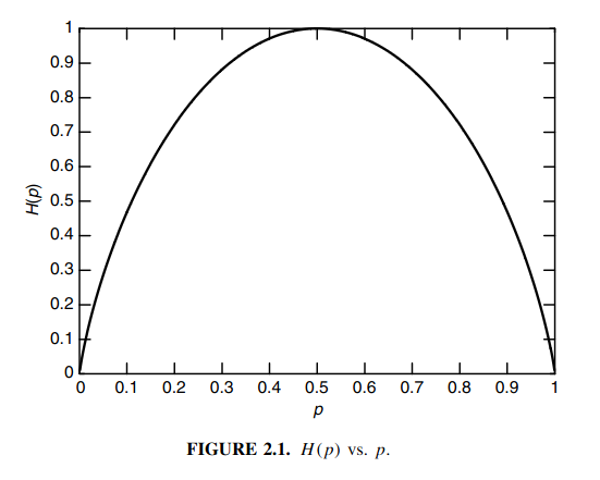
Example: Entropy of a coinflip for varying $p$. $H(p)$ is concave, vanishes at $p\in \{0,1\}$, and reaches its maximum of $1$ bit at $p=\frac{1}{2}$.

Nonnegativity of Entropy

For every $X$ it holds that:

$$H(X)\ge 0$$

Proof: For every $x$ we have $0\le p(x)\le 1$, so $\log \frac{1}{p(x)}\ge 0$. Entropy is an average of these terms.

2.2 Joint and Conditional Entropy

We can also define the entropy for multiple RVs:

Joint Entropy

For a pair of discrete random variables $(X,Y)\sim p(x,y)$, the joint entropy is

$$H(X,Y):=-\sum _{x\in \mathcal{X}}\sum _{y\in \mathcal{Y}}p(x,y)\log p(x,y)=-\mathbb{E}\left[\log p(X,Y)\right]$$

Note: This adds nothing new → $(X,Y)$ = single vector-valued RV

Conditional Entropy

For $(X,Y)\sim p(x,y)$, the conditional entropy of $Y$ given $X$ is the entropy of the conditional distributions, averaged over $X$:

$$\begin{array}{rl}H(Y\mid X)& :=\sum _{x\in \mathcal{X}}p(x)H(Y\mid X=x)\\ & =-\sum _{x\in \mathcal{X}}p(x)\sum _{y\in \mathcal{Y}}p(y\mid x)\log p(y\mid x)\\ & =-\sum _{x\in \mathcal{X}}\sum _{y\in \mathcal{Y}}p(x,y)\log p(y\mid x)\\ & =-\mathbb{E}\left[\log p(Y\mid X)\right]\end{array}$$

2.2.1 Chain Rule

$$H(X,Y)=H(X)+H(Y\mid X)$$

Proof: Since $p(x,y)=p(x)p(y\mid x)$,

$$\begin{array}{rl}H(X,Y)& =-\sum _{x,y}p(x,y)\log p(x)-\sum _{x,y}p(x,y)\log p(y\mid x)\\ & =-\sum _{x}p(x)\log p(x)-\sum _{x,y}p(x,y)\log p(y\mid x)\\ & =H(X)+H(Y\mid X)\end{array}$$

A shorter route: take expectations of both sides of $\log p(X,Y)=\log p(X)+\log p(Y\mid X)$.

Conditional Chain Rule

$$H(X,Y\mid Z)=H(X\mid Z)+H(Y\mid X,Z)$$

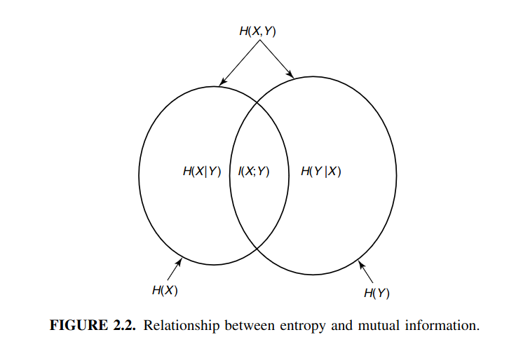
Note: In general $H(Y\mid X)\ne H(X\mid Y)$, but the differences always agree: $H(X)-H(X\mid Y)=H(Y)-H(Y\mid X)$.
→ this value is $I(X;Y)$, the mutual information (i.e. what they share)

2.3 Relative Entropy and Mutual Information

Relative Entropy (Kullback–Leibler Distance)

For two probability mass functions $p,q$ on $\mathcal{X}$, the relative entropy is

$$D(p\Vert q):=\sum _{x\in \mathcal{X}}p(x)\log \frac{p(x)}{q(x)}={\mathbb{E}}_p\left[\log \frac{p(X)}{q(X)}\right]$$

The following conventions apply: $0\log \frac{0}{0}=0$, $0\log \frac{0}{q}=0$, and $p\log \frac{p}{0}=\infty$ for $p>0$. So if some $x$ has $p(x)>0$ and $q(x)=0$, then $D(p\Vert q)=\infty$.

Note: $D(p\Vert q)=H(p,q)-H(p)$.

Cross entropy vs. Entropy $H(p,q)$ is not the same as $H(X,Y)$! $H(p,q)$ is called cross-entropy! With cross-entropy, we can compare two pmf's on the same $\mathcal{X}$.

Cross-Entropy Framing: if you code with a code designed for $q$ when the true distribution is $p$, you pay $H(p)+D(p\Vert q)$ bits on average instead of $H(p)$.

Note: $D$ is not a metric:

• not symmetric, i.e. $D(p\Vert q)\ne D(q\Vert p)$ in general)
• doesn’t satisfy the triangle inequality

Example: Asymmetry of knowledge about a coin. Assume we have $p(0)=1/2$ and $q(0)=1$ two coins.

• if we have a string of events $00000001$ → for sure must be $p$, since $q$ cannot have heads

• but for $00000$ → can only say it’s probably $q$.
  → this is reflected in $D(p\Vert q)=\infty$ but $D(q\Vert p)=1$.

Mutual Information

Let $X,Y$ have joint pmf $p(x,y)$ and marginals $p(x)$, $p(y)$. The mutual information $I(X;Y)$ is the relative entropy between the joint distribution and the product of the marginals:

$$\begin{array}{rl}I(X;Y)& :=\sum _{x\in \mathcal{X}}\sum _{y\in \mathcal{Y}}p(x,y)\log \frac{p(x,y)}{p(x)p(y)}\\ & =D(p(x,y)\Vert p(x)p(y))\\ & ={\mathbb{E}}_{p(x,y)}\left[\log \frac{p(X,Y)}{p(X)p(Y)}\right]\end{array}$$

2.4 Relationship Between Entropy and Mutual Information

Mutual Information and Entropy

The following properties hold:

$$\begin{array}{rl}I(X;Y)& =H(X)-H(X\mid Y)\\ I(X;Y)& =H(Y)-H(Y\mid X)\\ I(X;Y)& =H(X)+H(Y)-H(X,Y)\\ I(X;Y)& =I(Y;X)\\ I(X;X)& =H(X)\end{array}$$

Proof: Use $\frac{p(x,y)}{p(x)p(y)}=\frac{p(x\mid y)}{p(x)}$:

$$I(X;Y)=-\sum _{x,y}p(x,y)\log p(x)+\sum _{x,y}p(x,y)\log p(x\mid y)=H(X)-H(X\mid Y)$$

→ $I(X;Y)$ is the reduction in uncertainty about $X$ from knowing $Y$, and $X$ tells you exactly as much about $Y$ as $Y$ tells you about $X$.

• $I(X;X)=H(X)$ → entropy is sometimes called self-information.

2.5 Chain Rules for Entropy, Relative Entropy, and Mutual Information

Chain Rule for Entropy

Let $X_1,\dots ,X_n\sim p(x_1,\dots ,x_n)$. Then

$$H(X_1,X_2,\dots ,X_n)=\sum _{i=1}^{n}H(X_i\mid X_{i-1},\dots ,X_1)$$

We can repeatedly apply the two variable expansion rule to get the general chain rule:

• $H(X_1,X_2)=H(X_1)+H(X_2|X_1)$
• $H(X_1,X_2,X_3)=H(X_1)+H(X_2,X_3|X_1)=H(X_1)+H(X_2|X_1)+H(X_3|X_2,X_1)$

Proof: Write $p(x_1,\dots ,x_n)={\prod }_{i=1}^{n}p(x_i\mid x_{i-1},\dots ,x_1)$. Then

$$\begin{array}{rl}H(X_1,\dots ,X_n)& =-\sum _{x_1,\dots ,x_n}p(x_1,\dots ,x_n)\sum _{i=1}^n\log p(x_i\mid x_{i-1},\dots ,x_1)\\ & =-\sum _{i=1}^n\sum _{x_1,\dots ,x_i}p(x_1,\dots ,x_i)\log p(x_i\mid x_{i-1},\dots ,x_1)\\ & =\sum _{i=1}^{n}H(X_i\mid X_{i-1},\dots ,X_1)\end{array}$$

Conditional Mutual Information

The conditional mutual information of $X$ and $Y$ given $Z$ is the reduction in uncertainty about $X$ from learning $Y$ when $Z$ is already known:

$$I(X;Y\mid Z):=H(X\mid Z)-H(X\mid Y,Z)={\mathbb{E}}_{p(x,y,z)}\left[\log \frac{p(X,Y\mid Z)}{p(X\mid Z)p(Y\mid Z)}\right]$$

Note From exercise sheet 3 we know that $I(X;Y)$ has no relation to $I(X;Y|Z)$ in general.

Chain Rule for Mutual Information

$$I(X_1,X_2,\dots ,X_n;Y)=\sum _{i=1}^{n}I(X_i;Y\mid X_{i-1},\dots ,X_1)$$

Proof:

$$\begin{array}{rl}I(X_1,\dots ,X_n;Y)& =H(X_1,\dots ,X_n)-H(X_1,\dots ,X_n\mid Y)\\ & =\sum _{i=1}^{n}H(X_i\mid X_{i-1},\dots ,X_1)-\sum _{i=1}^{n}H(X_i\mid X_{i-1},\dots ,X_1,Y)\\ & =\sum _{i=1}^{n}I(X_i;Y\mid X_1,\dots ,X_{i-1})\end{array}$$

We can also define conditionality for relative entropy (i.e. Kullback-Leibler distance).

Conditional Relative Entropy

For joint pmfs $p(x,y)$ and $q(x,y)$, the conditional relative entropy is the relative entropy between the conditionals $p(y\mid x)$ and $q(y\mid x)$, averaged over $p(x)$:

$$D(p(y\mid x)\Vert q(y\mid x)):=\sum _{x}p(x)\sum _{y}p(y\mid x)\log \frac{p(y\mid x)}{q(y\mid x)}={\mathbb{E}}_{p(x,y)}\left[\log \frac{p(Y\mid X)}{q(Y\mid X)}\right]$$

Which we can also write as follows:

Chain Rule for Relative Entropy

$$D(p(x,y)\Vert q(x,y))=D(p(x)\Vert q(x))+D(p(y\mid x)\Vert q(y\mid x))$$

Proof: Factor both joints as marginal times conditional and split the logarithm:

$$\begin{array}{rl}D(p(x,y)\Vert q(x,y))& =\sum _{x,y}p(x,y)\log \frac{p(x)p(y\mid x)}{q(x)q(y\mid x)}\\ & =\sum _{x,y}p(x,y)\log \frac{p(x)}{q(x)}+\sum _{x,y}p(x,y)\log \frac{p(y\mid x)}{q(y\mid x)}\\ & =D(p(x)\Vert q(x))+D(p(y\mid x)\Vert q(y\mid x))\end{array}$$

Marginals

For two joint distributions $p,q$ on $\mathcal{X}\times \mathcal{Y}$, the divergence of the joints is at least the divergence of the marginals:

$$D(p(x,y)\Vert q(x,y))\ge D(p_x\Vert q_x)$$

with equality iff $p(y|x)=q(y|x)$ for all $x$ with $p(x)0$.

Note: this follows directly from the chain rule and $D(p\Vert q)\ge 0$.

2.6 Jensen’s Inequality and Its Consequences

From Jensen’s inequality we can derive things like QM-GM, AM-GM, etc… and it will be very useful in general.

Jensen's Inequality

If $f$ is convex and $X$ is a random variable, then

$$\mathbb{E}f(X)\ge f(\mathbb{E}X)$$

Note If $f$ is strictly convex and $\mathbb{E}f(X)\ge f(\mathbb{E}X)$ this implies $X=\mathbb{E}X$ with probability $1$, so $X$ is constant.

Proof: For discrete $X$, induct on the number $k$ of mass points. For $k=2$ the inequality is exactly the definition of convexity. For the inductive step, set $p_i^{\prime }=\frac{p_i}{1-p_k}$ for $i<k$. Then

$$\begin{array}{rl}\sum _{i=1}^k{p}_{i}f(x_i)& =p_{k}f(x_k)+(1-p_k)\sum _{i=1}^{k-1}{p}_i^{\prime }f(x_i)\\ & \ge p_{k}f(x_k)+(1-p_k)f\left(\sum _{i=1}^{k-1}{p}_i^{\prime }{x}_i\right)\\ & \ge f\left(p_k{x}_k+(1-p_k)\sum _{i=1}^{k-1}{p}_i^{\prime }{x}_i\right)=f\left(\sum _{i=1}^k{p}_i{x}_i\right)\end{array}$$

It holds more generally for any $\sum {\lambda }_{i}f(x)$ with $\sum {\lambda }_i=1$.

Information Inequality (or Gibb's)

For pmfs $p,q$ on $\mathcal{X}$,

$$D(p\Vert q)\ge 0$$

with equality if and only if $p(x)=q(x)$ for all $x$.

Proof: Let $A=\{x:p(x)>0\}$ be the support of $p$. Then

$$\begin{array}{rl}-D(p\Vert q)& =\sum _{x\in A}p(x)\log \frac{q(x)}{p(x)}\\ & \le \log \sum _{x\in A}p(x)\frac{q(x)}{p(x)}\\ & =\log \sum _{x\in A}q(x)\\ & \le \log \sum _{x\in \mathcal{X}}q(x)=\log 1=0\end{array}$$

→ this uses inverse Jensen’s (for concave) in the second step (as $\log$ is concave).

Equality If $D(p\Vert q)=0$, then $p,q$ are equal.

• as $\log$ is strictly concave, we only have the equals for a constant function.
• This means that $q(x)/p(x)=1$.

Nonnegativity of Mutual Information

For any random variables $X,Y$, $I(X;Y)\ge 0$ with equality if and only if $X$ and $Y$ are independent.

Proof: $I(X;Y)=D(p(x,y)\Vert p(x)p(y))\ge 0$, with equality if and only if $p(x,y)=p(x)p(y)$.

Nonnegativity of Conditional Relative Entropy

$D(p(y\mid x)\Vert q(y\mid x))\ge 0$ with equality if and only if $p(y\mid x)=q(y\mid x)$ for all $y$ and all $x$ with $p(x)>0$.

Nonnegativity of Conditional Mutual Information

$I(X;Y\mid Z)\ge 0$ with equality if and only if $X$ and $Y$ are conditionally independent given $Z$.

2.6.1 Entropy Inequalities

We can show that the uniform distribution maximises entropy.

Uniform Distribution Maximizes Entropy

$$H(X)\le \log |\mathcal{X}|$$

with equality if and only if $X$ is uniform on $\mathcal{X}$.

Proof: Let $u(x)=\frac{1}{|\mathcal{X}|}$. Then

$$0\le D(p\Vert u)=\sum _{x}p(x)\log \frac{p(x)}{u(x)}=\log |\mathcal{X}|-H(X)$$

New information cannot “hurt” → it always lowers entropy → we now know more.
Nothing about variable $Y$ could make us know less about $X$ on average.

Conditioning Reduces Entropy

$$H(X\mid Y)\le H(X)$$

with equality if and only if $X$ and $Y$ are independent.

Proof: $0\le I(X;Y)=H(X)-H(X\mid Y)$.

Note: This holds only on average. A particular observation can increase uncertainty, so $H(X\mid Y=y)>H(X)$ is possible.

Example: Let $(X,Y)$ have distribution:

• $P(X=1,Y=1)=0;P(X=2,Y=1)=3/4;P(X=1,Y=2)=\frac{1}{8};P(X=2,Y=2)=\frac{1}{8}$
• Then $H(X)=H\left(\frac{1}{8},\frac{7}{8}\right)\approx 0.544$ bit.
  • Observing $Y=1$ gives $H(X\mid Y=1)=0$, while observing $Y=2$ gives $H(X\mid Y=2)=1$ bit, which is more than $H(X)$.
• On average, though, $H(X\mid Y)=\frac{3}{4}\cdot 0+\frac{1}{4}\cdot 1=0.25$ bit, which is less.

Entropy of combined variables cannot be higher then the sum of entropies:

Independence Bound on Entropy

Let $X_1,\dots ,X_n\sim p(x_1,\dots ,x_n)$. Then

$$H(X_1,\dots ,X_n)\le \sum _{i=1}^{n}H(X_i)$$

with equality if and only if the $X_i$ are independent.

Proof: By the chain rule and the fact that conditioning reduces entropy,

$$H(X_1,\dots ,X_n)=\sum _{i=1}^{n}H(X_i\mid X_{i-1},\dots ,X_1)\le \sum _{i=1}^{n}H(X_i)$$

Equality $⟺$ each $X_i$ is independent of $(X_{i-1},\dots ,X_1)$ → equivalent to the $X_i$ being mutually independent.

2.7 Log Sum Inequality and Its Applications

Log Sum Inequality

For nonnegative numbers $a_1,\dots ,a_n$ and $b_1,\dots ,b_n$,

$$\sum _{i=1}^n{a}_i\log \frac{a_i}{b_i}\ge \left(\sum _{i=1}^n{a}_i\right)\log \frac{{\sum }_{i=1}^n{a}_i}{{\sum }_{i=1}^n{b}_i}$$

with equality if and only if $\frac{a_i}{b_i}$ is constant.
The conventions are $0\log 0=0$, $a\log \frac{a}{0}=\infty$ for $a>0$, and $0\log \frac{0}{0}=0$.

Proof: Without loss of generality, all $a_i,b_i>0$. The function $f(t)=t\log t$ is strictly convex, since $f^{\prime \prime }(t)=\frac{1}{t}\log e>0$.

• Apply Jensen’s inequality ${\sum }_i{\alpha }_{i}f(t_i)\ge f\left({\sum }_i{\alpha }_i{t}_i\right)$ with weights ${\alpha }_i=\frac{b_i}{{\sum }_j{b}_j}$ and points $t_i=\frac{a_i}{b_i}$:

$$\sum _i\frac{a_i}{{\sum }_j{b}_j}\log \frac{a_i}{b_i}\ge \frac{{\sum }_i{a}_i}{{\sum }_j{b}_j}\log \frac{{\sum }_i{a}_i}{{\sum }_j{b}_j}$$

• Multiplying through by ${\sum }_j{b}_j$ gives the claim.

Example: The log sum inequality gives a second proof that $D(p\Vert q)\ge 0$:

$$D(p\Vert q)=\sum _{x}p(x)\log \frac{p(x)}{q(x)}\ge \left(\sum _{x}p(x)\right)\log \frac{{\sum }_{x}p(x)}{{\sum }_{x}q(x)}=1\cdot \log \frac{1}{1}=0$$

Convexity of Relative Entropy

$D(p\Vert q)$ is convex in the pair $(p,q)$. That is, for pairs of pmfs $(p_1,q_1)$, $(p_2,q_2)$ and $0\le \lambda \le 1$,

$$D(\lambda p_1+(1-\lambda )p_2\Vert \lambda q_1+(1-\lambda )q_2)\le \lambda D(p_1\Vert q_1)+(1-\lambda )D(p_2\Vert q_2)$$

Proof: For each fixed $x$, apply the log sum inequality with $n=2$, $a_1=\lambda p_1(x)$, $a_2=(1-\lambda )p_2(x)$, $b_1=\lambda q_1(x)$, $b_2=(1-\lambda )q_2(x)$:

$$(\lambda p_1+(1-\lambda )p_2)\log \frac{\lambda p_1+(1-\lambda )p_2}{\lambda q_1+(1-\lambda )q_2}\le \lambda p_1\log \frac{\lambda p_1}{\lambda q_1}+(1-\lambda )p_2\log \frac{(1-\lambda )p_2}{(1-\lambda )q_2}$$

→ Summing over $x$ gives the result.

---

Concavity of Entropy

$H(p)$ is a concave function of $p$.

Proof: $H(p)=\log |\mathcal{X}|-D(p\Vert u)$, where $u$ is uniform. With $q=u$ fixed, $D(\cdot \Vert u)$ is convex, and it’s $-D(p\Vert u)$ → so $H$ is concave.
→ mixing two gases of equal entropy produces a gas with higher entropy.

Concavity and Convexity of Mutual Information

Let $(X,Y)\sim p(x,y)=p(x)p(y\mid x)$. Then $I(X;Y)$ is

• concave in $p(x)$ for fixed $p(y\mid x)$, and
• convex in $p(y\mid x)$ for fixed $p(x)$.

Note: channel capacity: $C={\max }_{p(x)}I(X;Y)$ is a omaximization of a concave function

TODO → Understand this better

2.10 Fano’s Inequality

We want to quantify the error when guessing the value of RV $X$, knowing only the value of RV $Y$.

• if $H(X\mid Y)=0$, i.e. $X$ is a function of $Y$ we can know with 0 error probability
• for other cases, the lower conditional entropy, the lower the guess
  → Fano’s inequality makes this quantitative.

Suppose we want to guess the value of RV $X$, using $Y$. We calculate $g(Y)=\hat{X}$, where $\hat{X}$ is an estimate of $X$ and takes on values in $\hat{\mathcal{X}}$.

• $\hat{\mathcal{X}}$ doesn’t need to be = to $\mathcal{X}$
• $g$ can be random.

Probability of Error

Let $X\to Y\to \hat{X}$, where $\hat{X}=g(Y)$ is an estimator of $X$ taking values in $\hat{\mathcal{X}}$. The estimator may be randomized, and $\hat{\mathcal{X}}$ need not equal $\mathcal{X}$. The probability of error is

$$P_e:=\mathrm{Pr}\{\hat{X}\ne X\}$$

Note: $X\to Y\to \hat{X}$ is a Markov Chain.

Fano's Inequality

For any estimator $\hat{X}$ with $X\to Y\to \hat{X}$ and $P_e=\mathrm{Pr}\{\hat{X}\ne X\}$,

$$H(P_e)+P_e\log |\mathcal{X}|\ge H(X\mid \hat{X})\ge H(X\mid Y)$$

Weaker but often more convenient forms are

$$1+P_e\log |\mathcal{X}|\ge H(X\mid Y)\text{and}{P}_e\ge \frac{H(X\mid Y)-1}{\log |\mathcal{X}|}$$

Proof: Define the error indicator $E=1$ if $\hat{X}\ne X$ and $E=0$ otherwise. Expand $H(E,X\mid \hat{X})$ with the chain rule in two ways:

$$\begin{array}{rl}H(E,X\mid \hat{X})& =H(X\mid \hat{X})+\underset{=0}{\underbrace{H(E\mid X,\hat{X})}}\\ & =\underset{\le H(P_e)}{\underbrace{H(E\mid \hat{X})}}+\underset{\le P_e\log |\mathcal{X}|}{\underbrace{H(X\mid E,\hat{X})}}\end{array}$$

The three marked bounds hold for the following reasons:

• $E$ is a function of $(X,\hat{X})$, so $H(E\mid X,\hat{X})=0$.
• Conditioning reduces entropy, and $E$ is binary, so $H(E\mid \hat{X})\le H(E)=H(P_e)$.
• Given $E=0$ we have $X=\hat{X}$, and given $E=1$ the entropy is at most $\log |\mathcal{X}|$, so

$$\begin{array}{rl}H(X\mid E,\hat{X})& =(1-P_e)H(X\mid \hat{X},E=0)+P_{e}H(X\mid \hat{X},E=1)\\ & \le (1-P_e)\cdot 0+P_e\log |\mathcal{X}|\end{array}$$

This proves $H(P_e)+P_e\log |\mathcal{X}|\ge H(X\mid \hat{X})$.
Data processing Inequality on $X\to Y\to \hat{X}$ gives $I(X;\hat{X})\le I(X;Y)$

• which is equivalent to $H(X\mid \hat{X})\ge H(X\mid Y)$.

Note: In particular, $P_e=0$ forces $H(X\mid Y)=0$.

Fano Without an Estimator

For any random variables $X,Y$, let $p=\mathrm{Pr}(X\ne Y)$. Then

$$H(p)+p\log |\mathcal{X}|\ge H(X\mid Y)$$

Proof: Apply Fano’s inequality with $\hat{X}=Y$.

If we force the estimator $\hat{X}$ to take values in $\mathcal{X}$, we can sharpen the bound:

Sharpened Fano

If the estimator takes values in $\mathcal{X}$, that is $\hat{X}:\mathcal{Y}\to \mathcal{X}$, then

$$H(P_e)+P_e\log (|\mathcal{X}|-1)\ge H(X\mid Y)$$

Proof: proof is the same as for Fano’s inequality, except for one bound:

• Given $E=1$ and $\hat{X}$, the value $X$ can only lie in the $|\mathcal{X}|-1$ values other than $\hat{X}$.
• So $H(X\mid \hat{X},E=1)\le \log (|\mathcal{X}|-1)$.

Fano’s inequality is sharp:

• For the worst possible $Y$, i.e. suppose there is no observation and $X\in \{1,\dots ,m\}$, and $p_1\ge \cdots \ge p_m$.
• The best guess is $\hat{X}=1$, with $P_e=1-p_1$, and Fano gives $H(P_e)+P_e\log (m-1)\ge H(X)$.

Collision Probability Bound

If $X$ and $X^{\prime }$ are i.i.d. with entropy $H(X)$, then

$$\mathrm{Pr}(X=X^{\prime })=\sum _{x}p(x{)}^2\ge 2^{-H(X)}$$

with equality if and only if $X$ is uniform.

Proof: The function $y\mapsto 2^y$ is convex, so by Jensen’s inequality $2^{\mathbb{E}\log p(X)}\le \mathbb{E}{2}^{\log p(X)}$. That is,

$$2^{-H(X)}=2^{{\sum }_{x}p(x)\log p(x)}\le \sum _{x}p(x)2^{\log p(x)}=\sum _{x}p(x{)}^2$$

Collision Bound for Different Distributions

Let $X\sim p$ and $X^{\prime }\sim r$ be independent on $\mathcal{X}$. Then

$$\mathrm{Pr}(X=X^{\prime })\ge 2^{-H(p)-D(p\Vert r)}\text{and}\mathrm{Pr}(X=X^{\prime })\ge 2^{-H(r)-D(r\Vert p)}$$

Proof: For the first bound,

$$\begin{array}{rl}{2}^{-H(p)-D(p\Vert r)}& =2^{{\sum }_{x}p(x)\log p(x)+{\sum }_{x}p(x)\log \frac{r(x)}{p(x)}}\\ & =2^{{\sum }_{x}p(x)\log r(x)}\\ & \le \sum _{x}p(x)2^{\log r(x)}=\sum _{x}p(x)r(x)=\mathrm{Pr}(X=X^{\prime })\end{array}$$

The inequality is Jensen’s inequality for the convex function $2^y$. The second bound follows by swapping the roles of $p$ and $r$.