2. Differentiation

TODO:

• Stetigkeit! wenn partial derivatives, die limit formulierung, etc…

• Def. 10.4: Differential $D{f}_{x_{\circ }}$ (totale Ableitung), mit Übung 10.5 (Eindeutigkeit) und

• 10.11: ${\partial }_{v}f(x_{\circ })$ existiert genau dann, wenn alle $g_j(s)=f_j(x_{\circ }+sv)$ in $s=0$ differenzierbar sind

2.1 Partielle Ableitung

Wir schneiden die Domain mit einer Ebene (ergibt eine normale Kurve), in welcher wir die “normale” Ableitung auswerten.

Differentiation

Es sei $U\subset {\mathbb{R}}^n$ offen mit Standardbasis $\{e_j{\}}_{j=1,\dots ,n}$, $x\in U$ und $f:U\subset {\mathbb{R}}^n\to \mathbb{R}$ eine Funktion.
Die Größe

$$\begin{array}{rl}& \underset{h\to 0}{\lim }\frac{f(x+h{e}_i)-f(x)}{h}\\ & =\underset{h\to 0}{\lim }\frac{f(x_1,x_2,\dots ,x_i+h,\dots ,x_n)-f(x_1,x_2,\dots )}{h}\\ & =:{\partial }_{e_i}f(x)={\partial }_{i}f(x)=\frac{\partial f}{\partial x_i}(x)=f_i(x)\end{array}$$

nennen wir die $i$-te partielle Ableitung von $f$ an der Stelle $x$.

Was fehlt?

• Wir können nur in die Basis-Kardinalrichtungen schauen, nicht in jede beliebige Richtung
• Ableitung gibt uns lineare Approximation ($f(y)=f(z)+f^{\prime }(z)(y-z)$ in 1D)
  → in ${\mathbb{R}}^2\to \mathbb{R}$ suchen wir eine Ebene, nicht eine Tangente.

---

Wir erweitern den Differentiationsbegriff also zur Richtungsableitung.

(Warum $U$ offen? Wir wollen keine komischen Rand-Effekte, dafür muss immer ein $ϵ$ Ball Platz haben.)

Directional Derivative

Let $U\subset {\mathbb{R}}^n$ be open, $x\in U$, $f:U\to \mathbb{R}$ and $v\in {\mathbb{R}}^n$. The directional derivative of $f$ at $x$ in direction $v$ is

$${\partial }_{v}f(x):=\frac{d}{ds}{|}_{s=0}f(x+sv)=\underset{s\to 0}{\lim }\frac{f(x+sv)-f(x)}{s}$$

provided the limit exists.

Note: Die Richtungsableitung ist die gewöhnliche 1D-Ableitung der Einschränkung $s\mapsto f(x+sv)$ auf die Gerade durch $x$ in Richtung $v$.

Note: Es gilt die Linearität ${\partial }_{\alpha v+\beta u}f(x_0)=\alpha {\partial }_v(x_0)+\beta {\partial }_u(x_0)$ → wir können jeden Vektor in Einheitsvektoren zerlegen und dann die normalen partiellen nutzen

• Partial derivatives are the special case $v=e_i$

2.1.1 Jacobian und Gradienten

Der Tangentenbegriff wird erweitert zu:

Total (all directions) Differentiable

Let $U\subset {\mathbb{R}}^n$ be open and $f:U\to {\mathbb{R}}^m$. $f$ is differentiable at $x\in U$ if there exists a linear map $L:{\mathbb{R}}^n\to {\mathbb{R}}^m$ such that

$$\underset{h\to 0}{\lim }\frac{\Vert f(x+h)-f(x)-L(h)\Vert }{\Vert h\Vert }=0$$

Note: $h$ ist hier ein Vektor im ${\mathbb{R}}^n$.
Note: im 1D ist $L(h)$ ja einfach nur $f^{\prime }(x)h$ da $\frac{f(x+h)-f(x)}{h}-\frac{f^{\prime }(x)}{h}=0$.

Wir können also umschreiben $f(x_0+x)=f(x_0)+L(x)+R(x)$ → für x dass sich $x_0$ nähert verhält sich $f$ wie eine lineare Funktion.

• der Fehler $R(x)$ muss in $o(|x|)$ sein.

Fehlerterm $R(h)$ konvergenz

Es muss gelten, dass

$$\underset{h\to 0}{\lim }\frac{||r(h)||}{||h||}=0$$

i.e. that $r(h)=o(||h||)$ damit $f$ differenzierbar ist.

Lokal Linear

Wenn für ein $f$ ein solches $L$ existiert, ist $f$ differenzierbar.
Wir können also Schlussfolgern, dass für differenzierbare $f$ gilt, dass sie sich lokal linear verhalten!
Der Gradientenvektor / die Jacobimatrix ist also lokal eine gute Approximation.

Wenn $f$ differenzierbar, existiert jede Richtungsableitung.

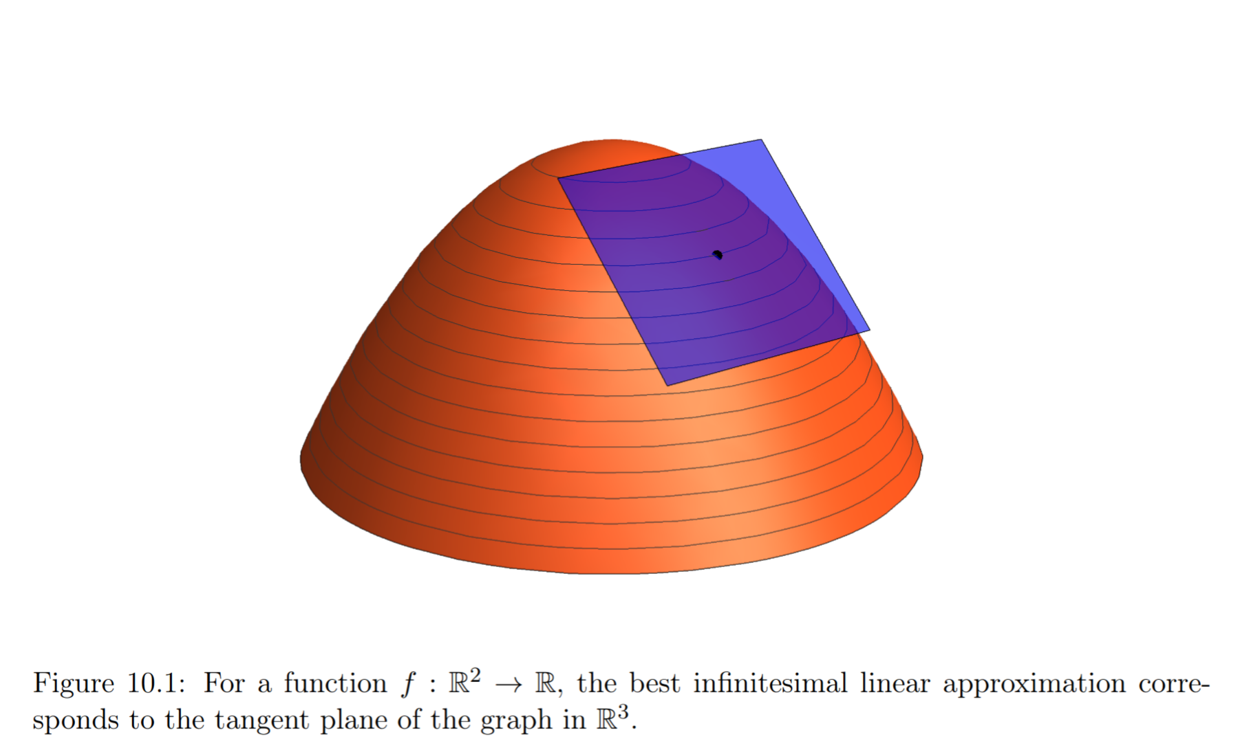
Das $L$ ist eine lineare Abbildung, i.e. eine Matrix!
→ Matrix = lineare “Plane”

Differentiable

$f$ is differentiable in $U$ if it is differentiable at every point of $U$.

Note: wir haben dann map $x\to d{f}_x(=L_x)$ von jedem Punkt zur Jacobi-Matrix.

---

Für jede Richtung (der Basis), repräsentiert die $i$-te Spalte der Matrix $L$ die Tangente in die Richtung $e_i$. Damit kann man dann alle anderen Richtungen “interpolieren”, i.e. exakt linear kombinieren.

Differential

$L$ is called the differential, (total) derivative or tangent map of $f$ at $x$, written

$$L=:D{f}_x(\text{also }df(x),D_{x}f,Df(x))$$

Da $L$ eine linear map ist, existiert eine Matrix welche diese eindeutig repräsentiert! Wir können $L$ also wie folgt als Matrix schreiben.

Jacobian Matrix

The linear map $L=D{f}_x$ is represented by the Jacobian matrix

$$J=\left(\begin{array}{cccc}{\partial }_1{f}^1& {\partial }_2{f}^1& \cdots & {\partial }_n{f}^1\\ ⋮& & & ⋮\\ {\partial }_1{f}^m& \cdots & \cdots & {\partial }_n{f}^m\end{array}\right)$$

In particular, $L$ is unique.

Note: Columns = directions, Rows = components $f^1,\dots ,f^m$ (i.e. welcher Input).
Uniqueness of the differential follows from this representation

Für eine Funktion welche nur eine Zeile hätte, fassen wir dies als den Gradientenvektor zusammen.

Gradient

For $f:U\subset {\mathbb{R}}^n\to \mathbb{R}$ the partial derivatives are collected in the gradient

$$\nabla f(x):=\left(\begin{array}{c}{\partial }_{1}f\\ {\partial }_{2}f\\ ⋮\\ {\partial }_{n}f\end{array}\right)$$

Note: Column vector; only for scalar-valued $f$

Note: the vector $\nabla f(x)$ points in the direction of the steepest ascent. It’s also exactly orthogonal to the Nivealinien.

Why is that?

• when we “zoom in” far enough, $f$ (for $f$ differentiable) starts to resemble a plane
  • i.e. it becomes linear
• Then, we take the partial derivatives (i.e. change in $x,y$ or however many inputs $f$ takes)
• Since $f$ is linear at this scale and 1-d derivatives already point to steepest direction
  • when it’s ascending → positive, when descending negative
• the combination of coordinates = steepest direction, since $f$ is linear.
• we can’t “miss a direction” since it’s linear

Once we have the gradient vector, we can oeasily calculate directional derivatives, using linear combination!

Directional Derivative using $\nabla$ or $J$

For $v\in {\mathbb{R}}^n$, s.t. $||v||=1$ (make sure it’s a unit vector, otherwise we don’t get the right scaling) and differentiable $f$, we have

$${\partial }_{v}f(x)=(\nabla f(x){)}^{\top }v=Jf(x)v$$

This makes it very easy to calculate directional derivatives, and it works since very zoomed in, the function behaves like a linear one.

2.1.2 Bedingungen für Ableitbarkeit

Differentierbarkeit ist für mehrdimensionale Funktionen eine deutlich striktere Bedingung als für 1 Variable.

• partielle Differenzierbarkeit ⇒ Stetigkeit ist nicht allgemein wahr

Example: Für $f(x,y)=\frac{xy}{x^2+y^2}$ mit $f(0,0)=0$ existieren beide partiellen Ableitungen, jedoch “matchen” sie nicht. $f$ ist also in $(0,0)$ nicht ableitbar.
→ Das liegt daran, dass die partiellen nur auf eine Achse anschauen was passiert, nicht auf den Diagonalen z.B.

$\exists$ Partial Derivatives $/⟹$ Differentiable

As shown in the example above, the existence alone of all partial derivatives does not guarantee that $f$ is differentiable.

Note: intuitively, we only check the “cardinal” directions. We’d have to check all (infinitely many of them) to be sure that all match.

What however does work is if we look at the output (codomain) and check if it’s component-wise differentiable there:

(Serra 9.6)

Let $U\subseteq {\mathbb{R}}^n$ be open and let $f:U\to {\mathbb{R}}^m$ be a function. $f_j$ is the j-th component of $f$.
Then $f$ is differentiable at $x_0$ if and only iff, for all $1\le j\le m$, $f_j$ is differentiable at $x_0$. In that case we have for all $v\in R^n$

$$(D{f}_{x_0}(v){)}_j=(D{f}_j{)}_{x_0}(v)$$

Proof: Condition for differentiability is $\frac{||R(x)||}{|x|}\to 0$. Since all norms are equivalent, take infinity-norm and transform it into component-wise statement.

The next statement is about the partials, i.e. the inputs of the function. They need to be $C^1$ for differentiability to hold.

Continuously Differentiable

Let $U\subset {\mathbb{R}}^n$ be open and $f:U\to {\mathbb{R}}^m$. If all partial derivatives $f_i$, $1\le i\le n$, exist and are continuous on $U$, then $f$ is called continuously differentiable and we write $f\in C^1(U,{\mathbb{R}}^m)$.

Note: By the previous theorem: $f\in C^1(U,{\mathbb{R}}^m)⟹f$ differentiable on $U$.

If all partials are continuously differentiable → $f$ is continuous

• technically you only need them to be bounded.

Note: We have the implication chain

$$C^1⟹\text{differentiable}⟹\text{all partials exist}$$

2.2 Höhere partielle Ableitungen

Die Menge der Ableitungen, welche wir nehmen müssen, steigt exponentiell (in der Dimensionalität der Funktion). Für jede Ableitungsrichtung, müssen wir erneut in alle Richtungen ableiten.

Second-Order Partial Derivatives

The partial derivatives $f_x(x,y)$, $f_y(x,y)$ are again functions of $x$ and $y$ and can be differentiated again. The four second-order partial derivatives are

$$\begin{array}{rlrl}\frac{{\partial }^{2}f}{\partial x^2}& =f_{xx}(x,y)=(f_x{)}_x(x,y)& \frac{{\partial }^{2}f}{\partial x\partial y}& =f_{yx}(x,y)=(f_y{)}_x(x,y)\\ \frac{{\partial }^{2}f}{\partial y^2}& =f_{yy}(x,y)=(f_y{)}_y(x,y)& \frac{{\partial }^{2}f}{\partial y\partial x}& =f_{xy}(x,y)=(f_x{)}_y(x,y)\end{array}$$

Note: Order convention: in $\frac{{\partial }^{2}f}{\partial x\partial y}$ the rightmost variable is differentiated first; in subscript notation $f_{yx}$ the leftmost subscript comes first, so $\frac{{\partial }^{2}f}{\partial x\partial y}=f_{yx}$.

$C^k$, $C^0$, $C^{\infty }$

Let $U\subset {\mathbb{R}}^n$ be open, $f:U\to {\mathbb{R}}^m$ and $k>1$. If all partial derivatives $f_i$, $1\le i\le n$, exist and lie in $C^{k-1}(U,{\mathbb{R}}^m)$, then $f$ is $k$-times continuously differentiable, written $f\in C^k(U,{\mathbb{R}}^m)$.

• $C^0(U,{\mathbb{R}}^m)$ denotes the class of all continuous functions $f:U\to {\mathbb{R}}^m$
• $C^{\infty }(U,{\mathbb{R}}^m)$ denotes the class of all smooth functions, i.e. $f\in C^k(U,{\mathbb{R}}^m)$ for all $k\ge 1$

Note: this is a recursive definition: $C^k$ is defined via $C^{k-1}$

2.2.1 Kommutativität der partiellen Ableitung

Es ist egal, ob wir zuerst in $x$ dann in $y$ oder $y$ dann $x$ ableiten (für $k$ Elemente gilt das nur für $k$-mal stetig differenzierbare Funktionen).

Schwarz

Let $U\subset {\mathbb{R}}^n$ be open and $f\in C^2(U,{\mathbb{R}}^m)$. Then

$${\partial }_j{\partial }_{i}f={\partial }_i{\partial }_{j}f\forall 1\le i,j\le n$$

Note: as stated before, this requires $C^2$.

Schwarz for $C^k$

Let $U\subset {\mathbb{R}}^n$ be open and $f\in C^k(U)$. Then for all $i_1,i_2,\dots ,i_k\in \{1,\dots ,n\}$ and every permutation $\sigma :\{1,\dots ,k\}\to \{1,\dots ,k\}$

$${\partial }_{i_1}{\partial }_{i_2}\cdots {\partial }_{i_k}f={\partial }_{i_{\sigma (1)}}{\partial }_{i_{\sigma (2)}}\cdots {\partial }_{i_{\sigma (k)}}f$$

Note this needs $k$-times continuously differentiable. Then the order of differentiation is irrelevant up to order $k$.

Using this rule, we can make our life easier. If in $y$ it’s a very complicated expression and with $x$ we get $0$, then doing $y$ then $x$ also yields $0$. No need to differentiate the complicated expression.

2.3 Continuously Differentiable Functions

Es gelten folgende Regeln.

Regularity of Sums, Products and Compositions

Let $U\subset {\mathbb{R}}^n$ be open, $f,g\in C^k(U,\mathbb{R})$, $h\in C^k(V,{\mathbb{R}}^n)$ with $V\subset {\mathbb{R}}^m$ open and $h(V)\subset U$. Then

• $f+g$ and $f\cdot g$ belong to $C^k$
• $f\circ h$ belongs to $C^k$

Für die Ableitung von composed functions gilt die Kettenregel, welche wir convenient mit Matrix-Multiplikation der Jacobians finden können.

Chain Rule

Let $k,m,n\ge 1$, $U\subset {\mathbb{R}}^n$ open and $V\subset {\mathbb{R}}^m$ open. If $f:U\to V$ is differentiable at $x$ and $g:V\to {\mathbb{R}}^k$ is differentiable at $f(x)$, then $g\circ f$ is differentiable at $x$ with

$$D(g\circ f{)}_x=D{g}_{f(x)}\circ D{f}_x$$

or component-wise

$$\frac{\partial (g\circ f{)}^j}{\partial x_i}(x)=\sum _{k=1}^m\frac{\partial g^j}{\partial y_k}(f(x))\frac{\partial f^k}{\partial x_i}(x)$$

This tells us “best linear approximation of the composition” is the composition of “the best linear approximation”.

Note: this only needs differentiability at $x$ and $f(x)$
→ Composition of differentials = product of Jacobian matrices

Example: Let $f,g:{\mathbb{R}}^2\to {\mathbb{R}}^2$ be given by $f(x_1,x_2)=\left(\begin{array}{c}{x}_1{x}_2\\ x_1+x_2\end{array}\right),g(y_1,y_2)=\left(\begin{array}{c}{y}_1+y_2\\ y_1{y}_2\end{array}\right)$ and evaluate at $x=(1,2)$, so $f(x)=(2,3)$.
The two Jacobians are

$$J_f(x)=\left(\begin{array}{cc}{\partial }_1{f}^1& {\partial }_2{f}^1\\ {\partial }_1{f}^2& {\partial }_2{f}^2\end{array}\right)=\left(\begin{array}{cc}{x}_2& x_1\\ 1& 1\end{array}\right)=\left(\begin{array}{cc}2& 1\\ 1& 1\end{array}\right)$$ $$J_g(y)=\left(\begin{array}{cc}{\partial }_1{g}^1& {\partial }_2{g}^1\\ {\partial }_1{g}^2& {\partial }_2{g}^2\end{array}\right)=\left(\begin{array}{cc}1& 1\\ y_2& y_1\end{array}\right),J_g(f(x))=J_g(2,3)=\left(\begin{array}{cc}1& 1\\ 3& 2\end{array}\right)$$

Note that $J_g$ is evaluated at $f(x)=(2,3)$, not at $x=(1,2)$. The product, with the computation of entry $(2,1)$ highlighted:

$$\underset{J_g(f(x))}{\underbrace{\left(\begin{array}{cc}1& 1\\ 3& 2\end{array}\right)}}\underset{J_f(x)}{\underbrace{\left(\begin{array}{cc}2& 1\\ 1& 1\end{array}\right)}}=\left(\begin{array}{cc}3& 2\\ 8& 5\end{array}\right)$$

If we look at the raw definition, without matrix-mult, we get the following, which still matches:

$$\begin{array}{rl}{\partial }_1(g^2\circ f)(x)& =({\partial }_1{g}^2)(f(x))\cdot {\partial }_1{f}^1(x)+({\partial }_2{g}^2)(f(x))\cdot {\partial }_1{f}^2(x)\\ & =3\cdot 2+2\cdot 1=8\end{array}$$

Chain Rule for $C^1$ Functions

Let $k,m,n\ge 1$, $U\subset {\mathbb{R}}^n$ open and $V\subset {\mathbb{R}}^m$ open. If $f\in C^1(U,{\mathbb{R}}^m)$, $g\in C^1(V)$ and $f(U)\subset V$, then

$${\partial }_i(g\circ f)=\sum _{k=1}^m\left(({\partial }_{k}g)\circ f\right)(x)\cdot {\partial }_i{f}^k(x)$$

This also tells us that $g\circ f$ is also in $C^1$ → only sum, product.

2.3 Mittelwertsatz

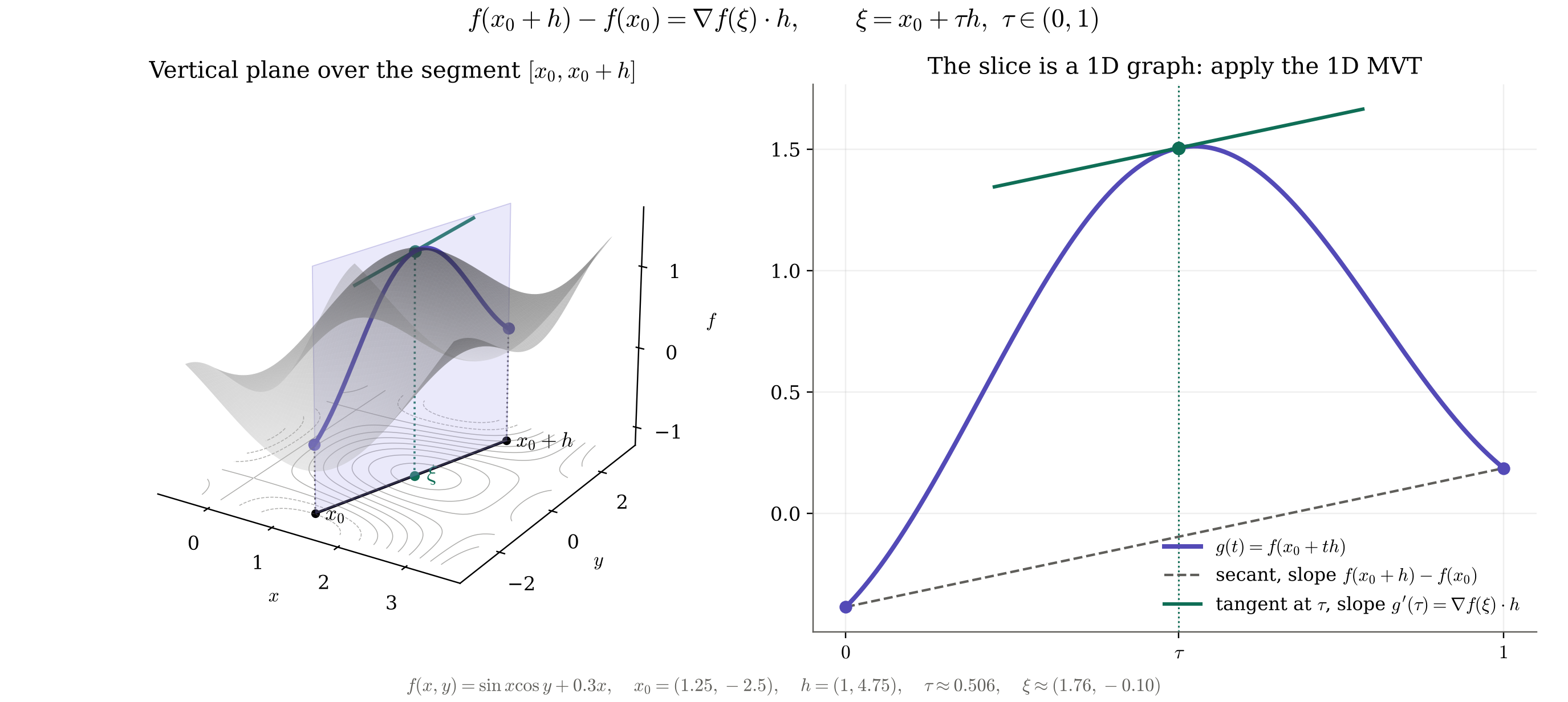
HIgher-Dimensional MVT (Serra 10.28)

Let $U\subset {\mathbb{R}}^n$ be open, and $f:U\to \mathbb{R}$, $f\in C^1$. Let $x_0\in U$ and $h\in {\mathbb{R}}^n$ s.t. $x_0+th\in U$ for all $t\in [0,1]$.
Then, there exists $\theta \in (0,1)$ s.t. for $ϵ=x_0+\theta h$, the following holds:

$$f(x_0+h)-f(x_0)={\partial }_{h}f(ϵ)=D{f}_{ϵ}(h)$$

What this means is that for such a function $f$, we can draw a vertical plane through the graph, cutting it in two points $f(x_0)$ and $f(x_0+h)$. On this plane, the 1-d MVT holds.

2.4 Taylor

Multi-Index

$\alpha =({\alpha }_1,\dots ,{\alpha }_n)\in {\mathbb{N}}_0^n$ is called a multi-index of length $|\alpha |$, where

$$|\alpha |:={\alpha }_1+\cdots +{\alpha }_n$$

We write $\beta \le \alpha$ if ${\beta }_i\le {\alpha }_i$ for all $i=1,\dots ,n$, and define the factorial

$$\alpha !:={\alpha }_1!\cdots {\alpha }_n!$$

For $f\in C^k$ and $|\alpha |\le k$ we set

$${\partial }^{\alpha }f:={\partial }_{x_1}^{{\alpha }_1}{\partial }_{x_2}^{{\alpha }_2}\cdots {\partial }_{x_n}^{{\alpha }_n}f={\partial }_1^{{\alpha }_1}{\partial }_2^{{\alpha }_2}\cdots {\partial }_n^{{\alpha }_n}f$$

This is just syntax sugar to make it easier to write.

Taylor

Let $U\subset {\mathbb{R}}^n$ be open, $f\in C^{k+1}(U)$, $k\ge 0$, $x_0\in U$ and $h\in {\mathbb{R}}^n$ such that $x_0+th\in U$ for all $t\in [0,1]$. Then

$$f(x_0+h)=\sum _{\alpha \in {\mathbb{N}}_0^n,|\alpha |\le k}{\partial }^{\alpha }f(x_0)\frac{h^{\alpha }}{\alpha !}+R_{k+1}f(x_0,h)$$

where the remainder is given by

$$R_{k+1}f(x_0,h):={\int }_0^1(k+1)(1-t{)}^k\sum _{\alpha \in {\mathbb{N}}^n,|\alpha |=k+1}\frac{{\partial }^{\alpha }f(x_0+th)}{\alpha !}{h}^{\alpha }dt=O(|h{|}^{k+1})$$

Note: ${\partial }^{\alpha }f$ is well-defined for $\alpha \in {\mathbb{N}}_0^n$ because of Schwarz (order doesn’t matter)
→ In the sum we basically have all possible partial derivatives up to that degree.

The big sum is basically Taylor grouped all together. We could also write it separated by $|\alpha |$, to get something looking more like traditional Taylor.

Example: For $k=2$, we have $\alpha$ that could be

$$\alpha \in \left\{\left(\begin{array}{c}0\\ 0\end{array}\right),\left(\begin{array}{c}1\\ 0\end{array}\right),\left(\begin{array}{c}0\\ 1\end{array}\right),\left(\begin{array}{c}2\\ 0\end{array}\right),\left(\begin{array}{c}1\\ 1\end{array}\right),\left(\begin{array}{c}0\\ 2\end{array}\right)\right\}$$ $$\begin{array}{rl}{T}_2=& f+f_x{h}_1+f_y{h}_2+f_z{h}_3\\ & +\frac{1}{2}{f}_{xx}{h}_1^2+\frac{1}{2}{f}_{yy}{h}_2^2+\frac{1}{2}{f}_{zz}{h}_3^2\\ & +f_{xy}{h}_1{h}_2+f_{xz}{h}_1{h}_3+f_{yz}{h}_2{h}_3\end{array}$$

2.5 Extremwerte

Critical Point

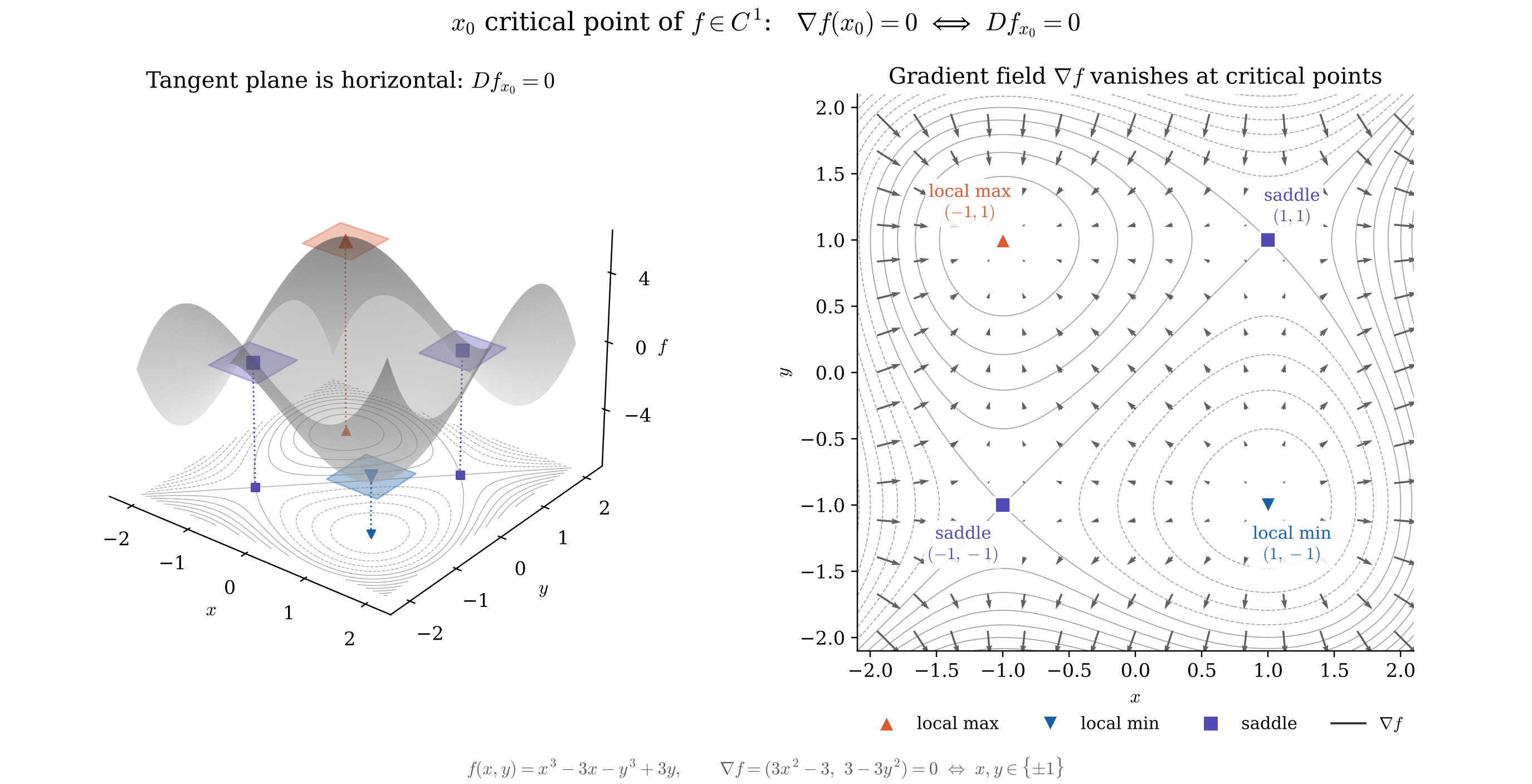
For $f\in C^1$, $x_0\in U$ is called a critical point of $f$ if the gradient of $f$ vanishes at $x_0$ (equivalently $D{f}_{x_0}$ is the zero map).

Note: this holds only for $f\in C^1$ → otherwise gradient 0 stops meaning flat.

Example: Such a critical point is reached at a plateau for example

Local Extrema

Let $f:\mathbb{D}\subset {\mathbb{R}}^n\to {\mathbb{R}}^m$ and $x_0\in D$.

1. $\exists \delta >0$ s.t. for all $x\in B_{\delta }(x_0)\cap \mathbb{D}$ we have $f(x_0)\ge f(x)$ we call $x_0$ a local maximum
2. $\exists \delta >0$ s.t. for all $x\in B_{\delta }(x_0)\cap \mathbb{D}$ we have $f(x_0)\le f(x)$ we call $x_0$ a local minimum
3. $x_0$ is called a lokale Extremstelle and $f(x_0)$ a lokaler Extremwert.

11.3 Interior Local Extrema are critical points

Let $x_0$ be a point where $f$ assumes a local extremum. Then ${\partial }_{i}f(x_0)$ for all $i=1,\dots ,n$. In other words, $\nabla f(x_0)=0$ and $x_0$ is a critical point of $f$.

NEXT
Vorzeichen der Hessematrix von Taylor → gibt Hinweis ob lokales Max/Min geben kann.