2. Polynominterpolation

2.1 Interpolation and Polynomials

2.1.1 Problem Setup and the Interpolation Condition

Want approximation in a linear subspace $V_n\subset V$ with $\dim V_n=n$ and basis $\mathrm{span}\{b_1,\dots ,b_n\}=V_n$:

$$f(x)\approx f_n(x)=\sum _{j=1}^n{\alpha }_j{b}_j(x)$$

→ not a least-squares fit: the interpolant passes through all data points $y_i=\tilde{f}(x_i)$.
for least squares we would want the one “closest” to all points equally.

$V$ has many different bases, each of which gives us different properties (numerical stability, ease of use, adding new datapoints, etc…)

Note: Taylor formula around $a$ is not suitable for numerical computation

• only approximates locally
• requires derivatives (hard or impossible to compute)

→ smoother $f$ ⇒ better convergence (approaches analytical)

2.1.5 The Space ${\mathcal{P}}_k$ and the Monomial Basis

Space of Polynomials

The space of polynomials of degree $\le k$, $k\in \mathbb{N}$, is

$${\mathcal{P}}_k:=\left\{x\mapsto {\alpha }_k{x}^k+{\alpha }_{k-1}{x}^{k-1}+\cdots +{\alpha }_{1}x+{\alpha }_0:{\alpha }_j\in \mathbb{K}\right\}$$

Properties of ${\mathcal{P}}_k$

${\mathcal{P}}_k$ is a vector space of dimension $k+1$, and ${\mathcal{P}}_k\subset C^{\infty }(\mathbb{R})$.

Proof: The monomials of degree $\le k$ form a basis of ${\mathcal{P}}_k$, so $\dim {\mathcal{P}}_k=k+1$. All polynomials are infinitely often continuously differentiable, hence ${\mathcal{P}}_k\subset C^{\infty }(\mathbb{R})$.

Uniqueness

A polynomial $p\in {\mathcal{P}}_k$ is uniquely determined by its values $y_i=p(x_i)$ at $k+1$ pairwise distinct nodes.

→ see Diskmath for proof

We can use the monomial basis to approximate a function. This corresponds to solving the following system: For $p_n(x)={\alpha }_n{x}^n+\cdots +{\alpha }_{1}x+{\alpha }_0$ through $y_0,\dots ,y_n$:

$$\left[\begin{array}{cccc}1& x_0& \cdots & x_0^n\\ 1& x_1& \cdots & x_1^n\\ ⋮& ⋮& \ddots & ⋮\\ 1& x_n& \cdots & x_n^n\end{array}\right]\left[\begin{array}{c}{\alpha }_0\\ {\alpha }_1\\ ⋮\\ {\alpha }_n\end{array}\right]=\left[\begin{array}{c}{y}_0\\ y_1\\ ⋮\\ y_n\end{array}\right]$$

→ Vandermonde matrix = very badly conditioned

• small perturbations will amplify a lot. Thus it’s bad for use with computers.
  ⇒ computed coefficients ${\alpha }_0,\dots ,{\alpha }_n$ are very inaccurate

Note: If we had infinite precision, we would get a correct answer (as guaranteed by the linear algebra). There is nothing wrong with the approach, only with computers.

Note: In the Vandermonde matrix, because $x^{11},x^{12},\dots$ look very similar on interval $[0,1]$, so in floating point precision they look linearly dependent.

• i.e. no inverse / we don’t span the space

This has a runtime of $O(n^2)$ for solving and $O(n)$ for evaluation.

Note: This is what polyfit computes internally (warns: RankWarning: Polyfit may be poorly conditioned.)

→ The fix is to use a better basis.

Extra: Condition Number

The condition number basically tells us how much a slight numerical error in the input affects the output → “amplification factor”

Condition Number

Let $f:X\to Y$ be a problem between normed spaces and let $x\in X$ with $x\ne 0$ and $f(x)\ne 0$. The relative condition number of $f$ at $x$ is

$$\kappa (x):=\underset{\delta \to 0}{\lim }\underset{\Vert \Delta x\Vert \le \delta }{\sup }\frac{\Vert f(x+\Delta x)-f(x)\Vert /\Vert f(x)\Vert }{\Vert \Delta x\Vert /\Vert x\Vert }$$

Note problem is well-conditioned at $x$ if $\kappa (x)$ is small and ill-conditioned if $\kappa (x)$ is large

• property of the problem not of the algorithm

Note: A backward-stable algorithm achieves a relative forward error of order $\kappa (x)\cdot {\epsilon }_{\text{mach}}$.

Condition Number of a Matrix

For an invertible matrix $A\in {\mathbb{C}}^{n\times n}$ and an induced matrix norm $\Vert \cdot \Vert$, the condition number of $A$ is

$$\kappa (A):=\Vert A\Vert \Vert A^{-1}\Vert$$

In the $2$-norm, ${\kappa }_2(A)=\frac{{\sigma }_{\max }(A)}{{\sigma }_{\min }(A)}$.

2.1.7 Evaluation via the Horner Scheme

Using the horner schema, we can evauluate with a monomial basis, using the least number of operations. It has a very small backwards error.

Horner Scheme

$$p(x)=(\cdots x(x({\alpha }_{n}x+{\alpha }_{n-1})+{\alpha }_{n-2})+\cdots +{\alpha }_1)x+{\alpha }_0$$

Note: equivalent to the normal polynomial evaluation, but is more numerically stable

numpy.polyval(p, x) evaluates it via Horner:

def horner(p, x):
    y = p[0]
    for i in range(1, len(p)):
        y = x * y + p[i]
    return y

2.2 Newton Basis and Divided Differences

Monomial basis: new data points → recomputing the whole interpolant.

WARNING

Why choose Newton? The Newton basis allows adding nodes without redoing everything.

By uniqueness (a polynomial of degree $k$ can be uniquely determined by $k+1$ datapoints), these polynomials coincide with those obtained naively.

2.2.2 The Newton Basis

Dividierte Differenzen sind diskrete Analoga der Taylor-Koeffizienten $f^{(k)}/k!$, und die Newton-Form ist das diskrete Analogon der Taylor-Entwicklung, mit Entwicklung um mehrere Punkte statt um einen.

Runtime:

• solving $O(n^2)$ via divided differences
• $O(n)$ für Auswertung
• $O(n)$ for adding new point! → the previous are not affected

Newton Basis

The polynomials

$$N_0(x):=1,N_1(x):=x-x_0,N_2(x):=(x-x_0)(x-x_1)$$

with

$$N_n(x):=\prod _{i=0}^{n-1}(x-x_i)$$

form a basis of ${\mathcal{P}}_n$.

The coefficients of $p_n(x)={\alpha }_0{N}_0(x)+\cdots +{\alpha }_n{N}_n(x)$ solve the lower triangular system (→ we expand it gradually, each depends only on previous)

$$\left[\begin{array}{cccc}1& 0& \cdots & 0\\ 1& (x_1-x_0)& \cdots & 0\\ ⋮& ⋮& \ddots & ⋮\\ 1& (x_n-x_0)& \cdots & {\prod }_{i=0}^{n-1}(x_n-x_i)\end{array}\right]\left[\begin{array}{c}{\alpha }_0\\ {\alpha }_1\\ ⋮\\ {\alpha }_n\end{array}\right]=\left[\begin{array}{c}{y}_0\\ y_1\\ ⋮\\ y_n\end{array}\right]$$

2.2.3 Divided Differences

Via divided differences, we can evaluate the coefficients of the polynomial quickly.

Divided Differences

$$y[x_i]=y_i,y[x_i,\dots ,x_{i+k}]=\frac{y[x_{i+1},\dots ,x_{i+k}]-y[x_i,\dots ,x_{i+k-1}]}{x_{i+k}-x_i}$$

They are computed with the tableau (each $>$ denotes one application of the recursion, basically DP on the coefficients):

$$\begin{array}{lllll}{x}_0& y[x_0]& & & \\ & & >y[x_0,x_1]& & \\ x_1& y[x_1]& & >y[x_0,x_1,x_2]& \\ & & >y[x_1,x_2]& & >y[x_0,x_1,x_2,x_3]\\ x_2& y[x_2]& & >y[x_1,x_2,x_3]& \\ & & >y[x_2,x_3]& & \\ x_3& y[x_3]& & & \end{array}$$

Which gives the final polynomial:

$$p(x)=y[x_0]+y[x_0,x_1](x-x_0)+\cdots +y[x_0,\dots ,x_n](x-x_0)\cdots (x-x_{n-1})$$

→ the coefficients are the leftmost diagonal in the tableau

Interpolation Error: the error for $n$ Stützstellen in $[a,b]$ is at most

$$\frac{(b-a{)}^{n+1}\Vert f^{(n+1)}{\Vert }_{\infty }}{(n+1)!}$$

→ Proof siehe Skript

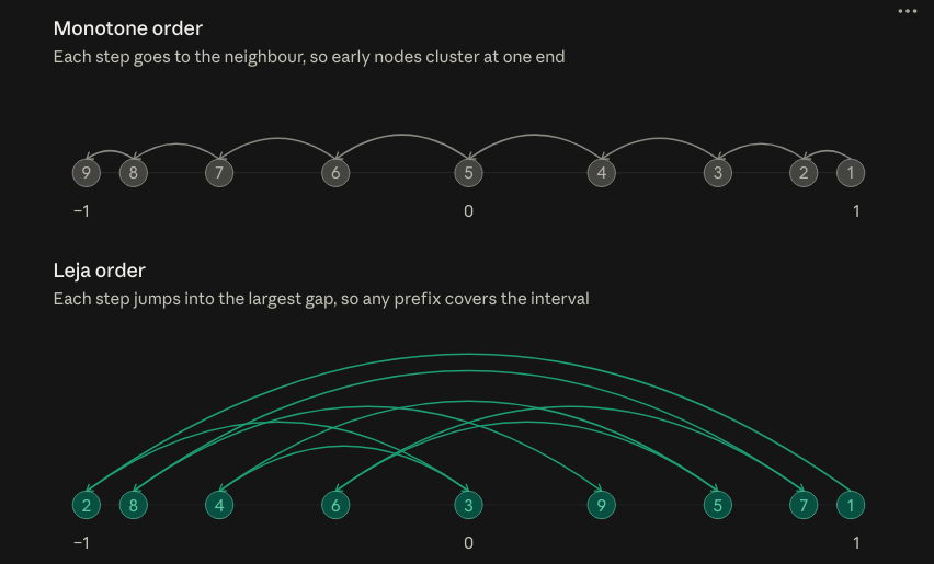
Note that for numerical stability, it matters a lot in which orders we consider the nodes! For divided difference we subtract $x_{i+k}-x_i$ in the denominator → this leads to blow-up if we choose nodes close together.
The Leja order maximises this distance →

2.3 Lagrange and Barycentric Interpolation

WARNING

Warum Lagrange? Wir wollen Basis die basically nichts zum rechnen hat

• Lagrange ist eine Cardinal basis mit $b_i(t_i)=1$ und $b_i(t_j)=0$ für $j\ne i$.

→ Die coefficients sind einfach die values $y_i$ selbst!

2.3.1 Lagrange Polynomials

Lagrange Polynomials

For nodes $x_0,\dots ,x_n\in \mathbb{R}$ define

$${\ell }_i(x)=\prod _{\begin{array}{c}j=0\\ j\ne i\end{array}}^n\frac{x-x_j}{x_i-x_j}$$

Diese Polynome formen eine Basis des Raums ${\mathcal{P}}_n$, wir können sie daher also auch verwenden um unsere Interpolation durchzuführen.

Properties:

1. ${\ell }_i(x_j)=0$ for all $j\ne i$
2. ${\ell }_i(x_i)=1$ for all $i$
3. $\mathrm{deg}{\ell }_i=n$ for all $i$
4. ${\sum }_{k=0}^n{\ell }_k(x)=1$ and ${\sum }_{k=0}^n{\ell }_k^{(m)}(x)=0$ for $m>0$

Proof: Lagrange ist eine Basis:

• Assume for contradiction $p(x)=\sum c_i\cdot {\ell }_i(x)=0$
• Da bei Lagrange coefficients $p(x_i)=c_i$ und hier $\forall xp(x)=0$ gilt
  • müssen alle Koeffizienten auch 0 sein.

2.3.2 The Barycentric Formula

Runtime:

• solving $O(n^2)$ via barycentric
• $O(n)$ für Auswertung
• $O(n)$ for adding new point!

With $L(x)=(x-x_0)\cdots (x-x_n)$ and

$${\lambda }_k=\prod _{j\ne k}\frac{1}{x_k-x_j},$$

we get $p(x)=L(x){\sum }_{k=0}^n\frac{{\lambda }_k}{x-x_k}{y}_k$.

For the constant polynomial $1$ this gives $1=L(x){\sum }_{k=0}^n\frac{{\lambda }_k}{x-x_k}$, hence the barycentric formula:

$$p(x)=\frac{{\sum }_{k=0}^n\frac{{\lambda }_k}{x-x_k}{y}_k}{{\sum }_{k=0}^n\frac{{\lambda }_k}{x-x_k}}$$

• extremely stable for $x\in [a,b]$
  • because orthogonal, no fighting on the $x_i$‘s?
• costs $O(n)$ per evaluation after precomputing the ${\lambda }_k$ in $O(n^2)$

→ weil es nur ein Polynom gibt mit Grad k für k+1 Terme, ist es auch sicher das richtige (egal wie weird es aussieht).

2.3.5 Fehler

The error depends only on the choice of nodes! The optimal choice are Chebychev-Nodes as we’ll see next.

Interpolation Error vs. Best Approximation

Let $f:[a,b]\to \mathbb{R}$ and $p$ its interpolation polynomial at $x_0,\dots ,x_n$. Then

$$\Vert f-p{\Vert }_{\infty }=\underset{x\in [a,b]}{\max }|f(x)-p(x)|\le (1+{\Lambda }_n)\underset{q\in {\mathcal{P}}_n}{\min }\underset{x\in [a,b]}{\max }|f(x)-q(x)|$$

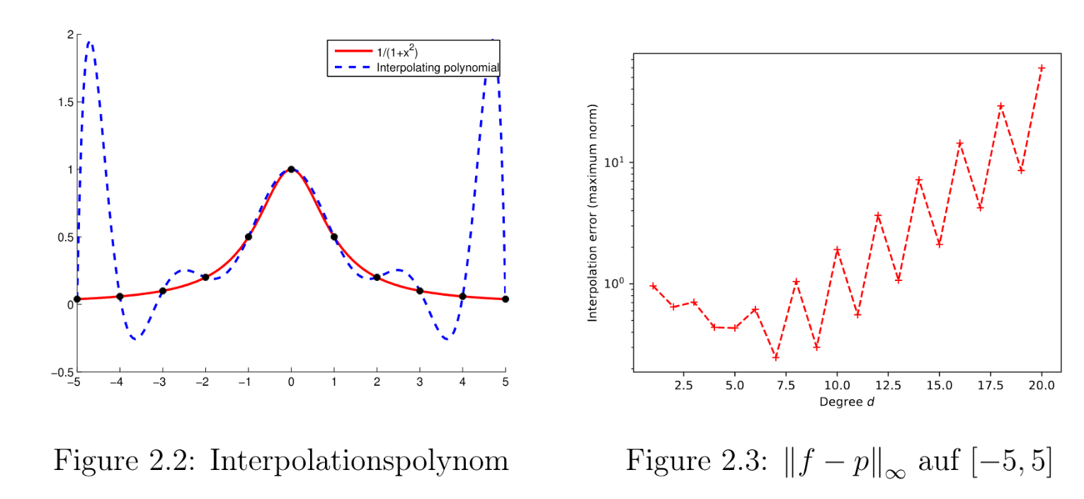
Note: Für gleichmässig auf $I$ verteilte Stützstellen gilt ${\Lambda }_n\approx \frac{2^{n+1}}{en\log n}$.

Deswegen sollten wir niemals gleichverteilte Stützstellen wählen → sie führen zum Runge-Phänomen.

2.4 Chebyshev Interpolation

Runtime

Method	Operations
Direct computation of $c_k$	$O((n+1{)}^2)$
Divided differences (comparison)	$O\left(\frac{n(n+1)}{2}\right)$
$c_k$ via FFT	$O(n\log n)$

Um das Runge-Phänomen zu vermeiden, wählen wir die Stützstellen so, dass am Rand mehr sind.

Chebyshev Polynomials of the First Kind

$$T_n(x)=\cos \left(n\arccos (x)\right),x\in [-1,1]$$

→ Schaut eigentlich nicht nach Polynomial aus???
ist es aber trotzdem → siehe Rekursionsformel.

$T_n$ is a polynomial of degree $n$, and for $x\in [-1,1]$:

1. $T_0(x)=1$, $T_1(x)=x$, $T_{n+1}(x)=2x{T}_n(x)-T_{n-1}(x)$
2. $|T_n(x)|\le 1$
3. $T_n\left(\cos \left(\frac{k\pi }{n}\right)\right)=(-1{)}^k$ for $k=0,1,\dots ,n$
4. $T_n\left(\cos \left(\frac{(2k+1)\pi }{2n}\right)\right)=0$ for $k=0,1,\dots ,n-1$

Proof (Recursion): We have

$$\cos ((n+1)t)=2\cos (nt)\cos (t)-\cos ((n-1)t)$$

Setting $\cos (t)=x$ gives the recurrence, which also shows that $T_n$ is a polynomial.

2.4.3 Chebyshev Nodes and Chebyshev Abscissae

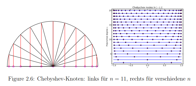
Nodes vs. Abscissae → kein wirklicher Unterschied, sind nur zwei Familien von Stützstellen.

Chebyshev Nodes

The $n+1$ Chebyshev nodes $x_0,\dots ,x_n$ in $[-1,1]$ are the zeros of $T_{n+1}$.

On an arbitrary interval $[a,b]$:

$$x_k=a+\frac{1}{2}(b-a)\left(\cos \left(\frac{2k+1}{2(n+1)}\pi \right)+1\right),k=0,\dots ,n$$

Chebyshev Abscissae

The $n-1$ Chebyshev abscissae $x_0,\dots ,x_{n-2}$ in $[-1,1]$ are the extrema of $T_n$; they are also the zeros of $U_{n-1}$. Depending on context, the points $-1$ and $1$ are added, giving $n+1$ Chebyshev abscissae.

On an arbitrary interval $[a,b]$:

$$x_k=a+\frac{1}{2}(b-a)\left(\cos \left(\frac{k}{n}\pi \right)+1\right),k=0,\dots ,n$$

Excluding the endpoints $a$ and $b$, $k=1,\dots ,n-1$.

LEMMA

When we use Chebychev Abscissae (second kind), the ${\lambda }_k=(-1{)}^k$ (for $k=0,n$, we have ${\lambda }_k=1/2$).
This makes computing the $\lambda$‘s extremely fast and easy (and stable).

The Chebyshev nodes/abscissae become denser towards the boundary of the interval
→ This is because at the boundary we observe these fluctuations = polynomial trying to “escape”

Note: für glatte Funktionen liefert Lagrange + Chebychev exponentiell schnelle Fehler-Konvergenz in $O(q^n)$ für $0<q<1$.

2.4.4 Orthogonality: Continuous and Discrete

Orthogonality I

The Chebyshev polynomials are orthogonal with respect to

$$⟨f,g⟩={\int }_{-1}^{1}f(x)g(x)\frac{1}{\sqrt{1-x^2}}dx$$

Proof: Substituting $x=\cos (\varphi )$, $dx=-\sin (\varphi )d\varphi =-\sqrt{1-x^2}d\varphi$:

$$\begin{array}{rl}⟨T_k,T_j⟩& =-{\int }_{\pi }^0\cos (k\varphi )\cos (j\varphi )d\varphi ={\int }_0^{\pi }\frac{1}{2}\left[\cos ((j-k)\varphi )+\cos ((j+k)\varphi )\right]d\varphi \\ & =\{\begin{array}{ll}0& j\ne k\\ \frac{\pi }{2}& j=k\ne 0\\ \pi & j=k=0\end{array}\end{array}$$

Orthogonality II

$T_0,\dots ,T_n$ are orthogonal in ${\mathcal{P}}_n$ with respect to the discrete inner product

$$(f,g)=\sum _{\ell =0}^{n}f(x_{\ell })g(x_{\ell }),$$

where $x_0,\dots ,x_n$ are the zeros of $T_{n+1}$.

Wie vorher gesehen, hängt der Fehler nur vom choice der Stützstellen ab.

$$\underset{x\in [-1,1]}{\max }|(x-x_0)\cdots (x-x_n)|$$

is minimal for $x_k=\cos \left(\frac{2k+1}{2(n+1)}\pi \right)$, the zeros of $T_{n+1}$. ${\Lambda }_n\approx \frac{2}{\pi }\log n\text{for }n\to \infty$

The Chebyshev abscissae are therefore the best possible choice and are preferred in practice (because of some extra properties).

Auswertung Chebychev

Der Clenshaw-Algorithmus zur Auswertung ist sehr stabil. Man kann damit $p(x)$ mithilfe einer Rückwärts-Rekursion berechnen.

Man kann Chebychev-Polynome sehr stabil berechnen, anhand dieser Rückwertsrekursion.

Clenshaw

Es gilt $p(x)=d_0-x{d}_1=\frac{1}{2}(d_0-d_2)$ mit $d_{n+2}=d_{n+1}=0$ und per Rekursion

$$d_k=c_k+(2x)d_{k+1}-d_{k+2}$$