5. Quadratur

Quadrature ist about computing the integral of a function. Sometimes we cannot analytically integrate → numerical approximation.

5.3 Grundbegriffe und -ideen

Quadraturformel (Def. 5.3.1)

Das Integral wird durch eine gewichtete Summe von Funktionswerten approximiert:

$$I(f):={\int }_a^{b}f(x)dx\approx \sum _{i=1}^n{w}_{i}f(c_i)=:Q_n(f;a,b)$$

wobei $w_i$ die Gewichte und $c_i\in [a,b]$ die Knoten der Quadraturformel sind.

Note: this is basically a Riemann sum, but we don’t always do it equidistant $h$‘s and we choose the weighs freely.

Fehler (Def. 5.3.2)

$$E(n):=\left|{\int }_a^{b}f(x)dx-Q_n(f;a,b)\right|$$

Algebraische Konvergenz: $E(n)=O(n^{-p})$, $p>0$. Exponentielle Konvergenz: $E(n)=O(q^n)$, $0\le q<1$.

Note: der Fehler kann nur für analytische glatte Funktionen und an $n$ anpassenden Order exponentiell konvergieren. Für alle dargestellten Methoden ist der Fehler algebraisch.

TODO: Why is this Lagrange?

use Riemann method → approximate using sum over some $n$ points with weights.

• can have weighetts $h$ for uniform with $h=1/(b-a)$
• the way we choose the value matters → take left, middle, right function v?
  • take polynomial, etc…
• we can choose the points → non-uniform to approximate with more points at more non-constant steps of the function

TODO: what is a cardinal basis (Lagrange ist cardinal basis)

Method order → has order d if perfectly approximates (error = 0) polynomials of degree d - 1 (if it has order 2 it also has order 1, but we take the highest such d)

1. Midpoint rule: $m=\frac{a+b}{2}$ Order 2

• it works not only for constants, but also for linear functions
  • left and right error cancel out!

2. Trapezoid rule: for $a,b$, find a linear function which goes through both of them

• then integrate that linear function
• $p(x)=f(a)+\frac{x-a}{h}(f(b)-f(a))$ → TODO this should be clear, liner interp
• Order 2 as well

3. Simpson’s Rule: we use 3 points and a deg 2 polynomial to approximate it

• use $a,b,m$
• Order 4

TODO If we fix these points, the $w$ are automatically given by lagrange????

• because for each section, we find the weights and the “polynomial” that approximates it
• then we have lagrange since those weights are exactly the “polynomial coefficients”

We divide the $[a,b]$ and use the 3 methods within the interval! Then we can make them non-equidistant to fix the issues of very spiky functions for example

4. Symmetric rules

• make sure the $c_i=-c_{n-1}$ and then the $w_i=-w_{n-i}$ are symmetric
• if rule is symmetric, then order is even
  • since if we have odd-degree polynomial, the highest degree monomial is odd
  • therefore the integral is = 0 and cancel out
  • this works since the quadrature is linear over the functions
    • we can “take out the odd-deg monomial” → integrates to be 0

Gauss-Lobatto → $a,b\in \{c_i|i\in \dots \}$ then order is $2s-2$

• midpoint rule → not Gauss-Lobatto
• Trapezoid, Simpson’s → are Gauss-Lobatto

5.4 Äquidistante Stützstellen

Wir können mit 3 verschiedenen Techniken stückweise Integrieren:

• Mittelpunkt
• Trapez
• Simpsons (Parabel)
  • summiert sogar $P_4$ korrekt, weil der höchste Term $x^3$ ist odd → cancelled beide Seiten aus = 0

Mittelpunkt → Cancelled links und rechts gleich aus, für “symmetrische Funktionen”

Die geben uns free ein extra Grad dazu quasi.

5.5 Nicht Äquidistante

Mit Gauss können wir optimale Stützstellen $c_i$‘s berechnen → funktioniert gut?

• Gauss-Legendre → a, b, nicht teil
  • TODO???
• Gauss-Radau = einer der beiden Endknoten a,b ist teil der Knoten
• Gauss-Lobatto = a, b sind teil der Knoten

wir finden die Knoten durch Konstruktion orthogonaler Basis im Polynom raum → Knoten sind dann die Nullstellen → wie bei Lagrange

alle Gauss-Gewichte sind positiv

Quadratur in ${\mathbb{R}}^d$ und dünne Gitter

→ visualise the smaller details adding up like in FFT

Nodale Basis vs. Hierarchische Basis
→ Like Gram-Schmidt hierarchisch?

• basisfunktion hängt von allen davor ab?

Hierarchisch → basically Gram-Schmidt + FFT Basis, immer mit Trapezregel das Gitter verfeinern

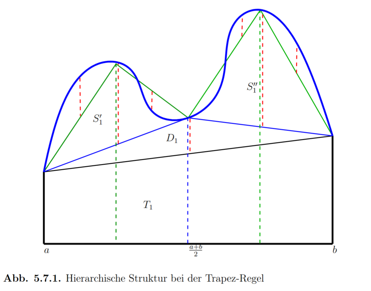
Gradinaru bild aus Vorlesung einfügen.

Smolyak konstruktion → verfeinerung in eine Richtung, mit hierarchischer Basis

Dünne Gitter = nur die Basen auf der Diagonale

TODO Verstehen die Grid Examples aus dem Skript → was heissen die Grid points