We are searching for the shortest walk in a graph. We can make the observation that the shortest walk is always a path (counting distance as the length of the walk, if we count edge-costs, then there might be negative ones).
Distance in a directed Graph
In the directed Graph , we define
For a shortest path problem that has additional state, such as cheats or similar, look at 0. Layered Graphs for an explanation.
Shortest Path - BFS
Runtime: .
If we want to find the shortest path from a vertex to another, we will need to determine the distances to all other reachable nodes, lest we overlook a “shortcut”.
The algorithm BFS (Breadth-First-Search) explores the graph in layers, first going to all adjacent vertices, then those adjacent to those, etc… We can easily disregard cycles (already visited nodes), as they would imply longer distances.
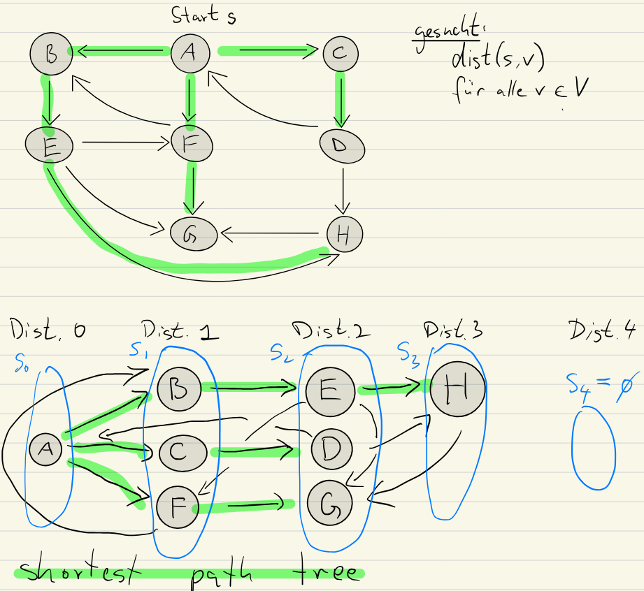
The tree at the bottom is called a shortest path tree. It represents the shortest distance from a vertex to all other reachable ones.
Levels
We can easily see here that there are multiple nodes at the same distance from as others.
Distance Levels
We can call this a level (of vertices at the same distance):
If there’s an edge from an to an , then as it increases distance by at most (and in an undirected graph , because it can also go back).
Algorithm How can we recursively compute the set , given ? We loop over the vertices, checking the following conditions for :
- We have to check that the vertex is not in previous levels (). If was already in a level closer to (start vertex), then that would be a shorter path.
- Successor of a vertex in We have to make sure is actually reachable in that distance , which by our previous formula is the case if there is an edge from a to .
Implementation with Queues
Using a queue (FIFO) for the implementation of BFS makes the algorithm more efficient and easier to implement.
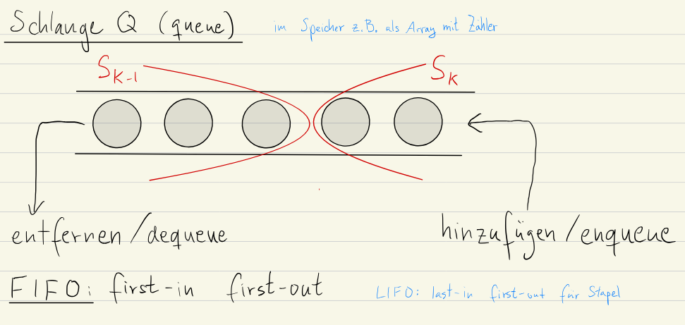
We maintain the list of levels “in the queue” instead of explicitly.
def bfs_shortest_paths(G, s):
  """Computes shortest path distances using BFS with a queue."""
  dist = {v: float('inf') for v in G}

  dist[s] = 0
  q = deque([s])  # Initialize queue with the source vertex
  parent = {} #dictionary to maintain shortest path tree

  while not q.empty():
    u = q.dequeue()

    for v in G[u]: # get adjacent nodes
        if dist[v] == float('inf'): # check v was not visited yet
          dist[v] = dist[u] + 1 # set distance
          parent[v] = u # u is parent of v

          q.enqueue(v)

return dist, parent # return distances and the shortest path tree- Initialisation:
- Set the distance to all vertices to in the
d[v]array. Set thed[s] = 0. - Initialise a Queue with
- Set the dictionary
parent = {}
- Set the distance to all vertices to in the
- Exploration:
- Dequeue the first element in the queue
- For all adjacent nodes with distance (not visited yet):
- Set the distance
d[u] = d[v] + 1 - add to the queue
- Set the
parent[u] = v.
- Set the distance
- Return: We return the distances and the shortest path tree
Runtime
The while loop runs over all vertices (exactly once as we check to prevent visiting multiple times), and in each operation we take .
The runtime of BFS is , we have constant time enqueue/dequeue and no set operations (needed without queue).
Enter and Leave Order
Same as with pre-/postordering, we can use enter-/leave-ordering here:
enterstep at which vertex is first encountered.leavestep at which vertex is dequeued
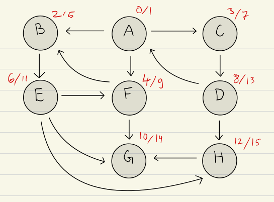
We can observe that:
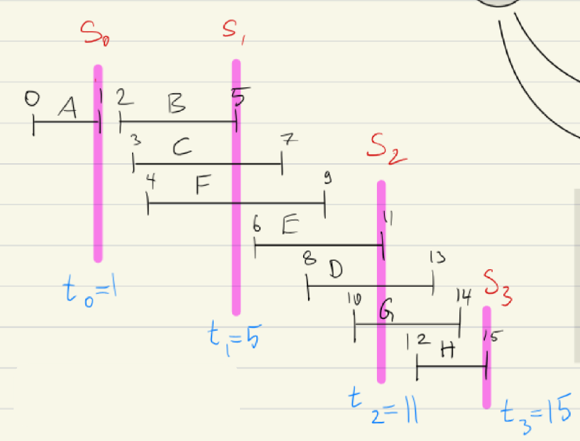
enter[v] < leave[v]This is fundamentalenterorderleave order: Within a given level, vertices enter the queue in the same order as they leave it in, this is due to the FIFO nature of a queue. Not true across different levels- Epochs (see Levels)
- is defined as the first time a vertex with distance is dequeued
- are the epochs in the execution of BFS
- We then have
We can prove BFS is correct using induction.
Checking for Bipartite Graph using BFS
We can use BFS to check if a graph is bipartite by checking if it can be two-coloured.
While traversing the tree, in each layer, we colour all vertices with the same. If we then encounter a vertex with the same colour during traversal, it’s not two-colourable.
public boolean isBipartite(int[][] graph) {
	int[] c = new int[graph.length];
	Queue<Integer> Q = new LinkedList<Integer>();

	int s = 0;

	c[s] = 1;
	Q.add(s);

	while (Q.size() > 0) {
		int u = Q.remove();

		for (int v : graph[u]) {
			if (c[v] == 0) {
				c[v] = (c[u] % 2) + 1;

				Q.add(v);
			} else {
				if (c[v] == c[u]) return false;
			}
		}

		if (Q.size() == 0) {
			for (int i = 0; i < c.length; i++) {
				if (c[i] == 0) {
					Q.add(i);
					c[i] = 1;
					break;
				}
			}
		}
	}

	return true;
}
Cheapest Walks in Weighted Graphs
Cost of a Walk
In a weighted graph () each edge is assigned a cost/weight. The cost of a walk is the sum of the weight of it’s edges: .
The cost of the cheapest path between is denoted as .
Negative Costs If we introduce the possibility of negative weights, there could be a cycle with a total negative cost. This means that we can’t have a “cheapest” path anymore as we can arbitrarily reduce the cost by just traversing the cycle more often.
A cheapest path in a weighted graph (without negative cycles) is the optimal substructure: any subpath is itself the cheapest path between it’s endpoints.
Triangle Inequality
The triangle inequality holds in a weighted graph:
This holds as if the path through was actually cheaper, then would be wrong.
Cheapest path recursively
We can define the cheapest path from to recursively thanks to the triangle inequality
The cheapest path from to is either if or the minimum cost among all paths that go from to some neighbour and then continue to from .
Cheapest Path Weighted Graph - Dijkstra’s
We assume that there are no negative edge-weights in the following.
We need to carefully consider the order of computation to avoid infinite loops or illegal access to values.
Dijkstra’s implicitly sorts the vertices by distance from the source and then uses only the previous ones in the calculation!
For Dijkstra’s, we needed to prove that for , the cheapest path from the source to is correctly computed by the recurrence
Vertices are considered in increasing order of their distances from the source.
To guarantee this, we maintain a set of vertices with definitely determined distance to the source.
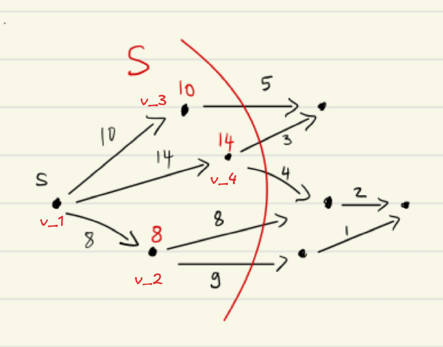
From this state, we would now choose the vertex with the minimum value, in this case it would be from using the edge with cost for a total of :
This works as the distance is equal to the true shortest path distance .
Proof
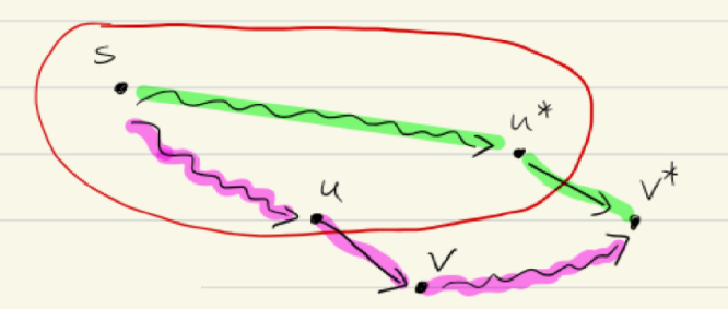
- Assume for contradiction that . This implies that there is a cheaper path from to that the one found by .
- Alternative Path Let be such a cheaper path from to . Since , this path must leave the set at some point. Let be the last vertex in along the path . Let be the first vertex outside along (note that might be itself).
- Cost
- Non-negative edge-costs since all edge costs are non-negative . Therefore .
- Contradiction
- We know that is the minimal path going from any node in to , therefore .
- …
- Since we chose such that is minimal (first vertex we considered in greedy algo), we have .
- This contradicts our assumption that is a cheaper path.
We conclude that .
Algorithm
Restrictions No negative edge-weights
Runtime
 def dijkstra(graph, start):
    # Initialize distances: all nodes are at "infinity" except the start node (0 distance to itself)
    distances = {node: infinity for each node in graph}
    distances[start] = 0

    # Create a priority queue to process nodes in the order of their distance from the start
    priority_queue = [(0, start)]  # (distance, node)

    while priority_queue is not empty:
        # Get the node with the smallest distance from the queue
        current_distance, current_node = pop the smallest item from priority_queue

        # For each neighboring node:
        for neighbor, weight in graph[current_node]:
            # Calculate the total distance to the neighbor
            distance = current_distance + weight

            # If this new distance is shorter than the previously known distance:
            if distance < distances[neighbor]:
                # Update the distance to this neighbor
                distances[neighbor] = distance

                # Add the neighbor to the queue for further exploration
                push (distance, neighbor) into priority_queue

    return distances
Use a MinHeap (a priority queue basically) as an efficient data structure in which we store the distances. Then we can quickly find the vertex with the currently cheapest cost and iterate.
The runtime is calculated from which gives .
Why the restriction on negative edge-weights?
The reason Dijkstra’s algorithm does not work on graphs with negative edges is that we exclude vertices from analysis once we visited them. As the distance to a vertex is not modified once we reached it, negative edges would violate the “safety property” we are exploiting.
In a non-negative graph, the triangle inequality holds and thus we mark visited vertices as safe. No path can be longer but cheaper. With negative edge-weights this no longer applies.
When is it better to use Dijkstra’s with an Array instead of a Priority Queue
We can also implement Dijkstra’s using an array instead of a priority queue.
Runtime:
extract_mintakes with an array ( in a MinHeap).decrease_keytakes in an array ( in a MinHeap) which is done maximum times for total runtime.
Therefore, the array implementation takes for (there are at most edges in a graph).
The MinHeap version takes .
In cases where the graph is very dense, i.e. , it makes more sense to use Dijkstra’s with an array.
Negative Edge-Weights Allowed - Bellman-Ford
Restrictions Negative edge weights allowed
Runtime
Detects negative weight cycles but can’t handle them (obviously, as cost is undefined there).
The idea of Bellman-Ford is to sort the vertices in the recursion by the number of edges in the cheapest path. We define the :
und and .
We then establish the recursion
The difficulty is calculating , but we can calculate good bounds.
Initialise the distances as
then we have -good bounds
We then improve the bounds from to by iterating over and setting
We have for thus this new for .
We have to perform this “relaxation” times, as this is the longest possible path from to for a connected graph with vertices.
Algorithm
It’s quicker to implement the edge-based approach, which iterates over all edges in each loop and then updates the distances immediately.
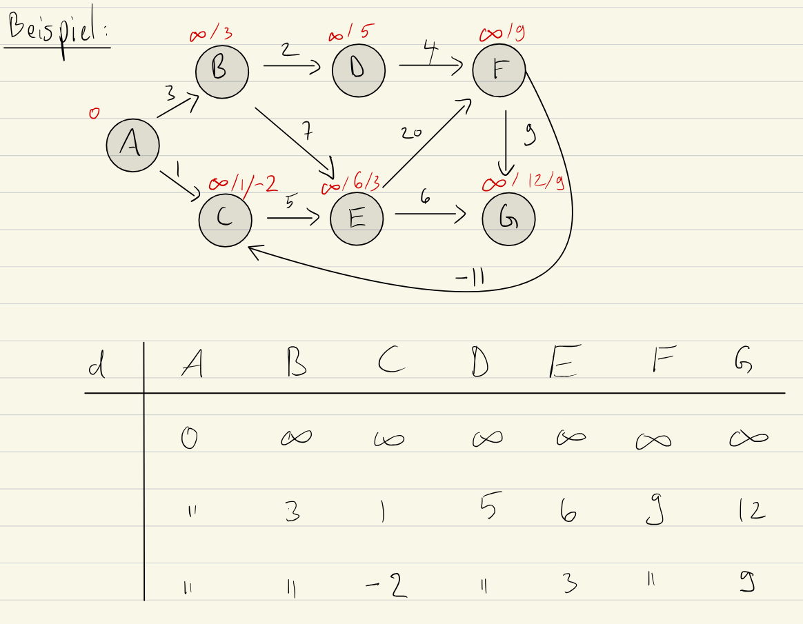
In this example, we start with , thus and the rest is . In the first relaxation step, we do:
Edge Based:
- : cost and , thus .
- : cost 1, thus
- : cost 2 and
- …
- : cost thus we update .
In the second relaxation step, we can improve on :
- : cost 5 and , thus
Vertex Based: - : cost 1, thus
- : cost -11, but we have thus we don’t update
- …
- now
In the second relaxation step, we can improve on : - : cost -11 and , thus
It depends on the order and method if one of these is faster, but they both iterate over all edges and thus find the same result.
EdgeBasedBellmanFord(G, s):
  Initialize distances: d[s] = 0, d[v] = ∞ for all v ≠ s

  for i = 1 to |V| - 1:  // Main relaxation loop
    for each edge (u, v) in E:
	  // If d[u] != Integer.MAX_VALUE in java
      if d[u] + c(u, v) < d[v]:
        d[v] = d[u] + c(u, v)

  for each edge (u, v) in E:  // Negative cycle detection
    if d[u] + c(u, v) < d[v]:
      return "Negative cycle detected"

  return d // Shortest path distances
We iterate over all edges in the “relaxation” thus the time complexity of that step is (the actual check is ).
As we relax (or for negative cycle check) times, the total runtime is .
Make B-F Faster: Toposort in a DAG
Restrictions No cycles
Runtime
In an acyclic graph, topological sorting is already an algorithm that gives us the most-efficient order to calculate the cost in.
This means that we can use Bellman-Ford to compute the shortest path in a single run (for a runtime of , which is linear time for graphs).
This is true because we know what edges come first (i.e. have no dependencies). We can therefore relax in that order and get correct distances after a single run.
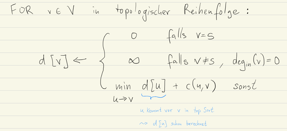
Go over the array and for each set the distance of it’s neighbours: if d[u] + c(u, v) < d[v] update d[v] to d[u] + c(u, v).
We can do this as if there’s a path from to , we have already calculated distance to before we go to (as it’s toposorted).
Negative Cycle detection with Bellman-Ford
We relax the edges one more time after times. If the distance to an edge decreased, there’s a negative cycle reachable from .
What is a relaxation actually?
Notice that we “relax” an edge when . In other words, there is a path from and such that it’s shorter than .
This means that our current upper-bound for the shortest distance to - , is too high as it violates the triangle inequality.
Therefore we set it to the lower value.