8. Eigenvalues and Eigenvectors

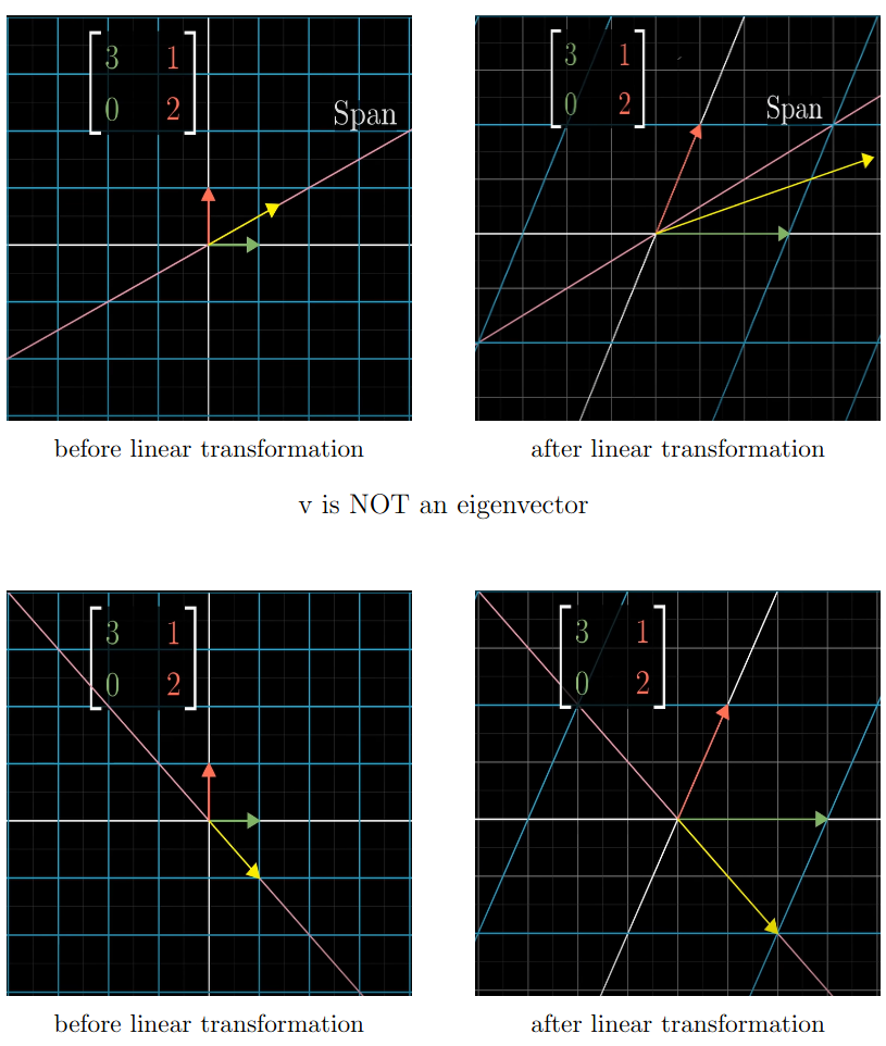
An eigenvalue, eigenvector pair is a scalar $\lambda \in \mathbb{R}$ and vector $v\in {\mathbb{R}}^n\setminus \{0\}$ such that $Av=\lambda v$. This means that the only transformation that $A$ applies to this vector is a scaling (or flipping by $-1$) (no turning, shifting, etc…).

For each eigenvalue, there are many eigenvectors (all colinear vectors).

If a matrix $A$ has the eigenvalue $0$, it means it collapses a set of vectors to $0$, meaning that the $N(A)\ne \{0\}$ and thus $A$ is not invertible. In the other side, if $0$ is not an EW of $A$, then $A$ is invertible.

8.1 Complex Numbers

Because Eigenvalues can be complex, we need some complex number manipulations.

We define $x^2=-1$ such that $\sqrt{-1}=i$ in the $\mathbb{C}$ complex numbers. This can be thought of as an extension field of $\mathbb{R}[x{]}_{x^2+1}$ (see DiskMath).

The operations in this field basically correspond to the polynomial operations we have seen, with $i$ being the “variable”:

• $(a+ib)+(x+iy)=(a+x)+i(b+y)$
• $(a+ib)(x+iy)=ax+i(ay+bx)+i^{2}by$ $=ax+i(ay+by)-by=$ $(ax-by)+i(ay+bx)$
• $(a+ib)(a-ib)=(a+ib)\overline{(a+ib)}=a^2+b^2$
• $\frac{a+ib}{x+iy}=\frac{(x-iy)(a+ib)}{(x-iy)(x+iy)}$ $=\frac{(ax+by)+i(bx-ay)}{x^2+y^2}$ $=(\frac{ax+by}{x^2+y^2})+i(\frac{by-ay)}{x^2+y^2}$

Given $z\in \mathbb{C}$ with $z=a+ib$ we have the following notation

• $\mathfrak{R}(a+ib)=\text{R}(a+ib):=a$ (the real part)
• $\mathfrak{I}(a+ib)=\text{Im}(a+ib):=b$ (the imaginary part)
• $|z|:=\sqrt{a^2+b^2}$ (the modulus, basically the length)
• $\overline{a+ib}:=a-ib$ (the complex conjugate of $z$)

There are some shortcuts

• $|z{|}^2=z\overline{z}$
• $z_1\cdot z_2=z_2\cdot z_1$ (commutative)
• $\overline{z_1+z_2}=\overline{z_1}+\overline{z_2}$
• $\frac{1}{z}=\frac{\overline{z}}{|z{|}^2}$

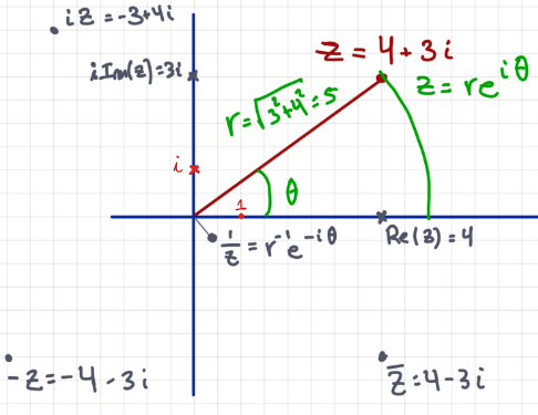
We can also define polar coordinates here $e^{i\theta }=\cos \theta +i\sin \theta$ which means $e^{i\pi }=-1$ (Euler’s Formula).

we can then express any $z\in \mathbb{C}$ as $z=r{e}^{i\theta }$ where $r\ge 0$ is the modulus and $\theta \in \mathbb{R}$ (restricted to $\theta \in [0,2\pi ]$) is an angle, the argument of $z$.

8.1.2 Fundamental Theorem of Algebra

Any degree $n$ non-constant $n\ge 1$ polynomial $P(z)=a_n{z}^n+a_{n-1}{z}^{n-1}+\cdots +a_{1}z+a_0$ with $a_n\ne 0$ has a (existance) zero: $\lambda \in \mathbb{C}$ such that $P(\lambda )=0$.

8.1.3 $n$ zeros

Any degree $n$ non constant ($n\ge 1$) polynomial $P(z)$ has $n$ zeros: ${\lambda }_1,\dots ,{\lambda }_n\in \mathbb{C}$, perhaps with repetitions such that $P(z)=a_n(z-{\lambda }_1)(z-{\lambda }_2)\dots (z-{\lambda }_n)$ The number of times $\lambda \in \mathbb{C}$ appears in this expansion is called the algebraic multiplicity of the zero.

Algebraic Multiplicity

The algebraic multiplicity of a root is the number of times it appears in the factorisation.

Example: If the algebraic multiplicity of ${\lambda }_2$ is $3$ then $(z-{\lambda }_2{)}^3|P(z)$.

We define one more new operation: $A^{\ast }={\overline{A}}^{\top }$ (the hermitian transpose). Which is conjugating each entry element-wise and then transposing. Note that ${\overline{A}}^{\top }=\overline{A^{\top }}$.

We have $||v|{|}^2=v^{\ast }v={\overline{v}}^{\top }v={\sum }_{i=1}^n\overline{v_i}{v}_i={\sum }_{i=1}^n|v_i{|}^2$. Note that for $\lambda ,v\in \mathbb{C}$ we have $||\lambda v|{|}^2=(\lambda v{)}^{\ast }(\lambda v)=(\overline{\lambda v}{)}^{\top }(\lambda v)$ where $\overline{\lambda v}=\overline{\lambda }\overline{v}$ thus at the end we get $||\lambda v|{|}^2=|\lambda {|}^2{v}^{\ast }v$. This is because $\overline{\lambda }\lambda =|\lambda {|}^2$ where that absolute value is the modulo for a complex number.

Tricks with Complex Numbers

Prove some $x\in \mathbb{C}$ is actually in $\mathbb{R}$:

• Show that $x=\overline{x}⟹x\in \mathbb{R}$

Tricks 2

If you have some expression $x_1+i{x}_2=y_1+i{y}_2$ we can separate this into:

• $x_1=y_1$
• $x_2=y_2$

because of the $i$.

8.1.999 (Example for Fibonacci from the Script)

We can express the Fibonacci formula $f_n=f_{n-1}+f_{n-2}$ as a matrix equation ${\mathbf{g}}_{n+1}=M{\mathbf{g}}_n$, where $M=\left[\begin{array}{cc}1& 1\\ 1& 0\end{array}\right]$.

Eigendecomposition: The eigenvalues ${\lambda }_1=\frac{1+\sqrt{5}}{2}$ (golden ratio $\varphi$) and ${\lambda }_2=\frac{1-\sqrt{5}}{2}$ are found, along with their eigenvectors $v_1=\left(\begin{array}{c}{\lambda }_1\\ 1\end{array}\right)$ and $v_2=\left(\begin{array}{c}{\lambda }_2\\ 1\end{array}\right)$ . These eigenvectors are independent since ${\lambda }_1\ne {\lambda }_2$ and thus they form a basis for ${\mathbb{R}}^2$.

Basis expansion: The initial state ${\mathbf{g}}_0$ is written as a linear combination of eigenvectors with coefficients $\pm \frac{1}{\sqrt{5}}$: $g_0=\frac{1}{\sqrt{5}}{v}_1-\frac{1}{\sqrt{5}}{v}_2$.

Power computation: Since $M^n{\mathbf{v}}_i={\lambda }_i^n{\mathbf{v}}_i$, we get the closed form: $F_n=\frac{1}{\sqrt{5}}\left[{\left(\frac{1+\sqrt{5}}{2}\right)}^n-{\left(\frac{1-\sqrt{5}}{2}\right)}^n\right]$

Worked Example: Tribonacci Numbers

Recurrence: $T_n=T_{n-1}+T_{n-2}+T_{n-3}$, with $T_0=0$, $T_1=0$, $T_2=1$.

Step 1: Companion matrix: $M=\left[\begin{array}{ccc}1& 1& 1\\ 1& 0& 0\\ 0& 1& 0\end{array}\right]$

Step 2: Characteristic polynomial: ${\lambda }^3-{\lambda }^2-\lambda -1=0$

This yields one real root (the “tribonacci constant” $\approx 1.839$) and two complex conjugate roots.

Follow the same procedure as before to get the closed form: $T_n={\alpha }_1{\lambda }_1^n+{\alpha }_2{\lambda }_2^n+{\alpha }_3{\lambda }_3^n$

8.2 Introduction to Eigenvalues and Eigenvectors

8.2.1 Eigenvalue, Eigenvector pair

Given $A\in {\mathbb{R}}^{n\times n}$ we say $\lambda \in \mathbb{C}$ is an eigenvalue of $A$ and $v\in {\mathbb{C}}^n\setminus \{0\}$ is an eigenvector of $A$ associated with the eigenvalue $\lambda$ when the following holds: $Av=\lambda v$

We call these an eigenvalue, eigenvector pair. If $\lambda \in \mathbb{R}$ then we call $\lambda$ a real eigenvalue. And the associated pair a real eigenvalue, eigenvector pair.

Note the zero vector was excluded. It is trivially always an eigenvector, thus we discard it.

How to Calculate EW, EV

We have $\lambda ,v$ and EW, EV pair and thus $v\ne 0$. \begin{align*} Av &= \lambda v \\ Av - \lambda v &= 0 \\ (A - \lambda I)v &= 0 \end{align*} This means that if $\lambda$ and $v$ are an eigenvalue, eigenvector pair, then $v$ is a non-zero element of the nullspace of the matrix $A-\lambda I$. Thus the matrix is not invertible $⟹\det (A-\lambda I)=0$. We can use this to calculate the EWs:

• By writing out $\det (A-\lambda I)=0$ we get a polynomial in $\lambda$. By solving for it, we get the EWs.
• From the EWs, we solve $Av={\lambda }_{i}v$ for all ${\lambda }_i$ we found before. Note that $v\ne 0$ must hold by definition.

8.2.3 Calculate real eigenvalues

Let $A\in {\mathbb{R}}^{n\times n}$. $\lambda \in \mathbb{R}$ is a real eigenvalue of $A$ if and only if $\det (A-\lambda I)=0$. A vector $v\in {\mathbb{R}}^n\setminus \{0\}$ is an eigenvector associated with the eigenvalue $\lambda$ if and only if $v\in N(A-\lambda I)$.

Note that a real EV always has a real EW associated with it. All eigenvalues are exactly the roots of the polynomial $\det (A-\lambda I)$. All the eigenvectors for ${\lambda }_i$ are the vectors $v\ne 0$, $v\in N(A-{\lambda }_{i}I)$, in the nullspace.

8.2.4 Polynomial degree

$\det (A-\lambda I)$ is a polynomial in $\lambda$ of degree $n$. The coefficient of the ${\lambda }^n$ term is $(-1{)}^n$.

8.2.5 Every matrix has an EW

Every matrix $A\in {\mathbb{R}}^{n\times n}$ has an eigenvalue (perhaps complex-valued).

Example: Eigenvalues of the $90^{\circ }$ degree counterclockwise rotation matrix $A=\left[\begin{array}{cc}0& -1\\ 1& 0\end{array}\right]$. The solutions to $0=\det (A-\lambda I)=-\lambda \cdot -\lambda -1\cdot (-1)={\lambda }^2+1$ which are ${\lambda }_1=i$ and ${\lambda }_2=-i$. The eigenvectors are given by $v_1=\left(\begin{array}{c}i\\ 1\end{array}\right)$ $v_2=\left(\begin{array}{c}-i\\ 1\end{array}\right)$. This makes sense because the only vector staying on it’s axis in a 2d rotation of a plane by $90^{\circ }$ is the vector pointing straight up, out from the plane.

EWs of an Orthogonal $Q$

Let $Q$ be an orthogonal matrix. If $\lambda \in \mathbb{C}$ is an eigenvalue of $Q$ then $|\lambda |=1$. The possible values for $\lambda$ are then $1,-1$ and all conjugate complex values with modulus $1$ for example $i,-i$.

This makes sense as $Q$ orthogonal only turns and doesn’t scale.

Complex EWs

Note that complex eigenvalues are possible even for real-valued matrices, as seen above.

8.2.8 Conjugate Pairs

Let $A\in {\mathbb{R}}^{n\times n}$. If $(\lambda ,v)$ is an eigenvalue, eigenvector pair, then $(\overline{\lambda },\overline{v})$ is an eigenvalue, eigenvector pair.

8.3 Properties

8.3.1 Properties of EWs, EVs (a)

If $\lambda$ and $v$ are an EW-EV pair of a matrix $A$, then, for $k\ge 1$, ${\lambda }^k$ and $v$ are an EW-EV pair of the matrix $A^k$.

Intuitively, $A$ on $v$ scales it by $\lambda$. Then scaling that already scaled $\lambda v$ by $A$ again gives us ${\lambda }^{2}v$, etc…

8.3.1 Properties (b)

Let $A$ be an invertible matrix. If $\lambda$ and $v$ are an EW-EV pair, then $\frac{1}{\lambda }$ and $v$ are an EW-EV pair of the matrix $A^{-1}$.

Proof: We have $Av=\lambda v$ thus $A^{-1}Av=\lambda A^{-1}v$ thus $\frac{1}{\lambda }v=\frac{1}{\lambda }\lambda A^{-1}v$ and we get $A^{-1}v=\frac{1}{\lambda }v$.

8.3.2 Linear independence

Let $A$ and $v_1,\dots ,v_k\in {\mathbb{R}}^n$ be the EVs of ${\lambda }_1,\dots ,{\lambda }_k\in {\mathbb{R}}^n$. If the ${\lambda }_1,\dots ,{\lambda }_k$s are all distinct then the EVs $v_1,\dots ,v_k$ are all linearly independent.

From this we know that we can write any vector as the linear combination of the eigenvectors, if they span the space.

8.3.3 Basis from Eigenvectors

Let $A$ with $n$ distinct real eigenvalues (meaning that the zeros of $\det (A-\lambda I)$ as described in Corollary 8.1.3 are all distinct, algebraic multiplicity $1$), then there is a basis of ${\mathbb{R}}^n$ made up of EVs of $A$

We also call this the Eigenbasis or a complete set of real EVs, which will come in handy later for Diagonalisation.

8.3.4 Characteristic Polynomial

$P(z)=(-1{)}^n\det (A-zI)=\det (zI-A)=(z-{\lambda }_1)(z-{\lambda }_2)\dots (z-{\lambda }_n)$ The polynomial $P(z)$ is called the characteristic polynomial of the matrix $A$. The eigenvalues ${\lambda }_1,\dots ,{\lambda }_n$ as they show up in the polynomial are not all distinct in general. The number of times an eigenvalue shows up is called the algebraic multiplicity of the eigenvalue.

Note that $\det (A-zI)$ and $\det (zI-A)$ have the same root and can both be used to find the eigenvalues. We can transform $\det (A-zI)=$ $(-1{)}^n\det ((-1)(A-zI))$ $=(-1{)}^n\det (zI-A)$ because $\det (\lambda A)={\lambda }^n\det (A)$.

The characteristic polynomial is always monic, the polynomial $\det (A-zI)$ has a leading $(-1)$ if the degree is odd. Therefore working with the characteristic one is easier.

Note as defined later, the geometric multiplicity is the $\dim (N(A-{\lambda }_{i}I))$.

8.3.4 (2)

The trace of $A$ is defined as $\text{Tr}(A)={\sum }_{i=1}^n{A}_{ii}$.

8.3.5 Eigenvalues of the transpose

The eigenvalues of $A$ are the same ones as those of $A^{\top }$.

WARNING: The eigenvectors are not the same in general however.

8.3.6 Trace and Determinant

Let $A\in {\mathbb{R}}^{n\times n}$ and ${\lambda }_1,\dots ,{\lambda }_n$ its $n$ eigenvalues. Then $\det (A)={\prod }_{i=1}^n{\lambda }_i(1)$and $\text{Tr}(A)={\sum }_{i=1}^n{\lambda }_i(2)$

Be careful to include each eigenvalue as often as their algebraic multiplicity in these sums/products. You can use this to double check calculations.

Explanation (1): The eigenvalues describe how much each eigenvector is scaled. Thus by multiplying the scaling of each dimension, we can figure out the volume of the unit cube which is the determinant.

Explanation (2): The Lemma 8.3.6 is quite surprising, since the determinant and trace are $\in \mathbb{R}$ where the eigenvalues in general must not be? It holds because complex eigenvalues $z_1,z_2$ always show up in pairs: $z_1=\overline{z_2}$. And because $z_1\cdot \overline{z_1}=a^2+b^2$ and $z_1+\overline{z_1}=2a$.

8.3.7 Properties of the trace

$\text{Tr}(AB)=\text{Tr}(BA)$ and $\text{Tr}(ABC)=\text{Tr}(CBA)=\text{Tr}(BAC)$ The trace is commutative, which makes sense as addition is element-wise.

Warnings

1. $A$ and $A^{\top }$ share eigenvalues not eigenvectors
2. The eigenvalues of $A+B$ are not the eigenvalues of $A$ + those of $B$. They aren’t correlated.
3. The eigenvalues of $AB$ or $BA$ are not easily computed from those of $A$ and $B$.
4. Gaussian Elimination does not preserve EWs or EVs. This means the EVs and EWs depend on the representation of the matrix, not on the subspaces they define.

Some extra Notes

Special cases

Real Symmetric matrices always have real eigenvalues. Real Skew-Symmetric matrices always have imaginary (or zero) eigenvalues!

$AB=BA$ ($A,B$ commute) then they share an EW-EV

Assume $AB=BA$.

If $\lambda ,v$ an EW-EV pair of $A$ then $A(Bv)=(AB)v=B(Av)=\lambda Bv$ thus $Bv$ is an eigenvector of $A$. Then $Bv$ is a multiple of some $v$ of that EW $\lambda$ (easiest to see for $A$ complete set of real EVs) $⟹$ $Bv={\lambda }^{\prime }v$ thus that $v$ is also an EV of $B$

Thus both $A$ and $B$ share an EV: $(A+B)v=Av+Bv=\lambda v+{\lambda }^{\prime }v=(\lambda +{\lambda }^{\prime })v$ then $A+B$ also has that EV.

Eigenvalues of $M+cI$

For an eigenvalue $\lambda$ of $M$, $\lambda +c$ is a real eigenvalue of the matrix $M+cI$. This is easily verified by calculation.

Intuitively this makes sense as by adding $cI$ were increasing the values on the diagonal, meaning we have to increase the value of $\lambda$ by the same amount so it makes $0$ again.

Example If we have $A$ with eigenvalues $0,1,2$ then $I+A^2$ has eigenvalues? We have ${\lambda }^2$ eigenvalues of $A^2$ by lemma script. Thus $0,1,4$ are EWs. Then $1+{\lambda }^2$ are the eigenvalues of $I+A^2$ thus $1,2,5$ are the EWs.

Find Eigenvectors of a $\lambda$

The eigenvectors of an eigenvalue are those and exactly those vectors in $v\ne 0$, $v\in N(A-\lambda I)$.

Special Case: EW $\lambda =0$ $\iff$ A not invertible

We know the EV are in the $N(A-\lambda I)$ because they solve the formula $Av=\lambda v⟹Av-\lambda v=0⟹(A-\lambda I)v=0$. Thus $v$ is in the nullspace of $(A-\lambda I)$.

If $A$ is not invertible, then it will have an EV of $0$, which means that there is an EV solving $(A-0\cdot I)v=0⟹Av=0$. Thus $v$ is in the nullspace of $A$.

If the EV $0$ has algebraic multiplicity of more than $1$ the nullspace needs to have more than $1$ dimension, otherwise it won’t have a complete set of EVs.