9. Diagonalisable Matrices and the SVD

We know from 8. Eigenvalues and Eigenvectors that given $n$ EV we can build a basis of ${\mathbb{R}}^n$ if the matrix has $n$ distinct real eigenvalues.

What happens in the case where some eigenvalues are repeated? Can we still build a basis of ${\mathbb{R}}^n$? Example:

$$A=\left[\begin{array}{cc}0& 1\\ 0& 0\end{array}\right]B=\left[\begin{array}{cc}0& 0\\ 0& 0\end{array}\right]$$ $$\det (A-\lambda I)={\lambda }^2\det (B-\lambda I)={\lambda }^2$$ $${\lambda }_1=0,{\lambda }_2=0{\lambda }_1=0,{\lambda }_2=0$$ $$\dim (\mathbf{N}(A-0I))=1\dim (\mathbf{N}(B-0I))=2$$

Both matrices have the eigenvalue $0$ with algebraic multiplicity 2. But $B$ has $0$ with geometric multiplicity $2$ as well, thus the multiplicities match and we can build a basis as we’ll see later in a theorem. “In general when there is an eigenvalue $\lambda$ with algebraic multiplicity larger than 1, it can be that $N(A-\lambda I)$ is of large enough dimension to find enough linearly independent eigenvectors.”

From EWs to Diagonalisable Matrices

Whenever we have a basis of ${\mathbb{R}}^n$ that consists of real eigenvectors of $A$ we can change the basis of the row and column space to view $A$ as a diagonal matrix, which is then easy to invert.

9.1.1 Diagonalisation

Let $A\in {\mathbb{R}}^{n\times n}$. Suppose that $A$ has eigenvectors $v_1,\dots ,v_n\in {\mathbb{R}}^n$ that form a basis of ${\mathbb{R}}^n$. For $i\in \{1,\dots ,n\}$ let ${\lambda }_i$ be the eigenvalue associated to $v_i$. Let $V$ be the matrix whose columns correspond to the eigenvectors $v_1,\dots ,v_n$. Then, $A=V\Lambda V^{-1}$where $\Lambda$ is a diagonal matrix with ${\Lambda }_{ii}={\lambda }_i$ (and ${\Lambda }_{ij}=0$ for all $i\ne j$).

Proof Since $v_1,\dots ,v_n$ forms a basis, the vectors are independent and $V^{-1}$ exists. We then verify that $V^{-1}AV=\Lambda$. For any $1\le j\le n$ the $j$-th column of the matrix $V^{-1}AV$ is given by $(V^{-1}AV{)}_j=(V^{-1}AV)e_j=V^{-1}A{v}_j=V^{-1}{\lambda }_j{v}_j={\lambda }_j{V}^{-1}{v}_j={\lambda }_j{e}_j$ since $V^{-1}{v}_j=V^{-1}V{e}_j=ej$. Since for any $1\le j\le n$ ${\lambda }_j{e}_j$ is the $j$-th column of $\Lambda$ we are done.

9.1.2 Diagonalisable Matrix

A matrix $A$ is called diagonalisable if there exists an invertible matrix $V$ such that $V^{-1}AV=\Lambda$ where $\Lambda$ is a diagonal matrix.

9.1.3 Complete set of real eigenvectors

If given a matrix $A$ we can build a basis of ${\mathbb{R}}^n$ with eigenvectors of $A$ we say that $A$ has a complete set of real eigenvectors.

Examples A diagonal matrix $D$ has eigenvalues which are the diagonal entries of $D$ and a full set of eigenvectors $e_1,\dots ,e_n$. Note distinct eigenvalues imply distinct vectors, distinct vectors don’t imply distinct eigenvalues. There can be an eigenvalue with geometric multiplicity $>1$ such that it’s eigenvectors span more than $1$ dimension.

Example The eigenvalues of a $n\times n$ triangular matrix are the diagonals. However, it might not have a complete set of real eigenvectors. $A=\left[\begin{array}{cc}1& 1\\ 0& 1\end{array}\right]$ does not for example.

9.1.6 EVs, EWs of a Projection Matrix

Let $P$ be the projection matrix onto the subspace $U\subset {\mathbb{R}}^n$. Then $P$ has two eigenvalues, $0$ and $1$, and a complete set of real eigenvectors.

Proof Let $m$ be the dimension of $U$. Let $u_1,\dots ,u_m$ be an orthonormal basis of $U$ and $w_1,\dots ,w_{n-m}$ be an orthonormal basis of $U^{\perp }$. $P{u}_k=1u_k$ (thus EW 1) and $P{w}_k=0w_k$ (thus EW 0). The geometric multiplicities match the algebraic ones here, thus $P$ has a complete set of real eigenvectors.

9.17. Similar Matrices

We say that $A\in {\mathbb{R}}^{n\times n}$ and $B\in {\mathbb{R}}^{n\times n}$ are similar matrices if there exists an invertible matrix $S$ such that $B=S^{-1}AS$.

9.1.8 Similar Matrices share Eigenvalues

Similar matrices $A$ and $B=S^{-1}AS$ have the same eigenvalues. The matrix $A$ has a complete set of real eigenvectors if and only if $B$ does.

Proof $\lambda ,v$ EW, EV pair for matrix $A$ iff $Av=\lambda v\iff \lambda S^{-1}v=S^{-1}Av=S^{-1}AS{S}^{-1}v=B(S^{-1}v)$.

9.1.10 Geometric Multiplicity

Given a matrix $A\in {\mathbb{R}}^{n\times n}$ and an eigenvalue $\lambda$ of $A$ we call the dimension $\dim (N(A-\lambda I))$ the geometric multiplicity of $\lambda$.

9.1.11 Geometric and Algebraic Multiplicities match

A matrix has a complete set of real eigenvectors if all its eigenvalues are real and the geometric multiplicities are the same as the algebraic multiplicities of all it’s eigenvalues.

Example $I$ has eigenvalue $1$ with geometric multiplicity $n$ ($\dim (N(I-1\cdot I))=n$) and algebraic multiplicity $n$ (As the characteristic polynomial of $I$, $P(z)=(z-1)(z-1)\dots (z-1)$ with that repeated $n$ times).

9.2 Symmetric Matrices and the Spectral Theorem

9.2.1 Spectral Theorem

Any symmetric matrix $A\in {\mathbb{R}}^{n\times n}$ has $n$ real eigenvalues and an orthonormal basis of ${\mathbb{R}}^{n\times n}$ consisting of it’s eigenvectors.

9.2.2 Diagonalisation

For any symmetric matrix $A\in {\mathbb{R}}^{n\times n}$ there exists an orthogonal matrix $V\in {\mathbb{R}}^{n\times n}$ (whose columns are the eigenvectors of $A$) such that $A=V\Lambda V^{\top }$where $\Lambda \in {\mathbb{R}}^{n\times n}$ is a diagonal matrix with the eigenvalues of $A$ in it’s diagonal (and $V^{\top }V=I$).

This decomposition is called an eigen-decomposition.

9.2.4 Rank of Symmetric Matrix

The rank of a real symmetric matrix $A$ is the number of non-zero eigenvalues (counting repetitions).

9.2.5 Rank of any A

For general $n\times n$ non-symmetric matrices, the rank is $n-\dim (N(A))$ so it’s $n$ minus the geometric multiplicity of $\lambda =0$.

9.2.6 Recover A from EVs, EWs

Let $A$ be a real $n\times n$ symmetric matrix and let $v_1,\dots ,v_n$ be an orthonormal basis of eigenvectors of $A$ (the columns of matrix $V$ in diagonalisation) and ${\lambda }_1,\dots ,{\lambda }_n$ the associated eigenvalues. Then $A={\sum }_{k=1}^n{\lambda }_i{v}_i{v}_i^{\top }$

We now show some Lemmas useful for the proof of the Spectral Theorem.

9.2.7 Orthogonal EVs for distinct EWs

Let $A\in {\mathbb{R}}^{n\times n}$ be a symmetric matrix and ${\lambda }_1\ne {\lambda }_2\in \mathbb{R}$ be two distinct eigenvalues of $A$ with corresponding eigenvectors $v_1,v_2$. Then $v_1$ and $v_2$ are orthogonal.

Proof ${\lambda }_1{v}_1^{\top }{v}_2=(A{v}_1{)}^{\top }{v}_2=v_1^{\top }{A}^{\top }{v}_2=v_1^{\top }(A{v}_2)={\lambda }_2{v}_1^{\top }{v}_2$ Thus $v_1^{\top }{v}_2$ must be $0$.

9.2.8 All EVs of Symmetric Matrices are Real

Let $A\in {\mathbb{R}}^{n\times n}$ be a symmetric matrix and $\lambda \in \mathbb{C}$ be an eigenvalue of $A$, then $\lambda \in \mathbb{R}$.

Proof $v\in {\mathbb{C}}^n$ be EV of $\lambda$. Thus we have $Av=\lambda v$. Since $A$ is symmetric we have $A^{\ast }=A$. $\overline{\lambda }||v|{|}^2=\overline{\lambda }{v}^{\ast }v=(\lambda v{)}^{\ast }v=(Av{)}^{\ast }v=v^{\ast }{A}^{\ast }v=v^{\ast }Av\text{ (uses }{A}^{\ast }=A\text{) }=v^{\ast }\lambda v=\lambda ||v|{|}^2$ Since $v\ne 0$, then $||v||\ne 0$ and so $\lambda =\overline{\lambda }$ thus $\lambda \in \mathbb{R}$.

9.2.9

Every symmetric matrix $A\in {\mathbb{R}}^{n\times n}$ has a real eigenvalue $\lambda$.

Proof of the Spectral Theorem

The Spectral Theorem is proven by induction . For any $1\le k\le n$ there are $k$ orthogonal eigenvectors of $A$. We want to show that this holds for $k=n$.

B.C.: For $k=1$: Since $A$ symmetric, we have a real eigenvalue and thus vector, which we normalise to get $k=1$ orthogonal eigenvectors. I.H.: We assume the statement and show that it holds for $k+1$. I.S.: We have $v_1,\dots ,v_k$ $k$ orthonormal eigenvectors and ${\lambda }_1,\dots ,{\lambda }_k$ he respective EWs. We also have $u_{k+1},\dots ,u_n$ an orthonormal basis of the orthogonal complement to the span of $v_1,\dots ,v_k$. We define $V_k$ the matrix as $V_k=\left[\begin{array}{cccccc}|& & |& |& & |\\ v_1& \dots & v_k& u_{k+1}& \dots & u_n\\ |& & |& |& & |\end{array}\right]$ and then define $B=V^{\top }AV$.

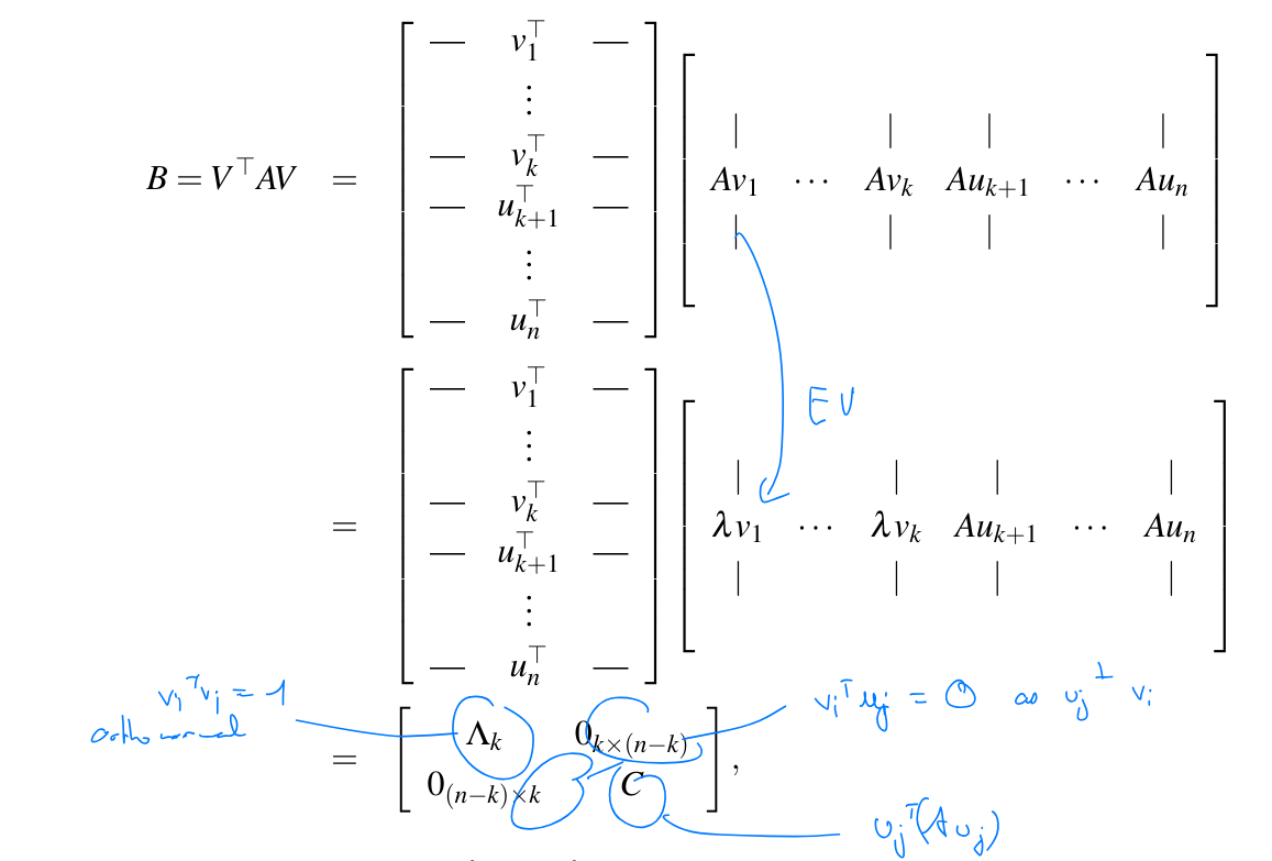
We note that $C$ is a $(n-k)\times (n-k)$ symmetric matrix. Therefore it has one real eigenvalue ${\lambda }_{k+1}$ and a real eigenvector $y\in {\mathbb{R}}^{n-k}$. We define $w_i=\{\begin{array}{ll}0& \text{if }i\le k\\ y_{i-k}& \text{if }i>k\end{array}$ which means we’re basically lifting $y$ into ${\mathbb{R}}^n$. We have 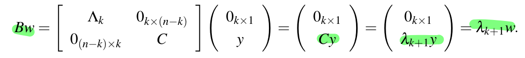Define $v_{k+1}:=Vw$. Since $V$ is orthogonal it has $V^{\top }$ inverse thus $A=VB{V}^{\top }$. Thus $A{v}_{k+1}=VB{V}^{\top }{v}_{k+1}=VBw=V{\lambda }_{k+1}w={\lambda }_{k+1}{v}_{k+1}$. Thus $v_{k+1}$ is an eigenvector of $A$.

Applications

9.2.10 Rayleigh Quotient

Given a symmetric matrix $A\in {\mathbb{R}}^{n\times n}$ the Rayleigh Quotient defined for $x\in {\mathbb{R}}^n\setminus \{0\}$, as $R(x)=\frac{x^{\top }Ax}{x^{\top }x}$attains it’s

• maximum at $R(v_{\text{max}})={\lambda }_{\text{max}}$
• minimum at $R(v_{\text{min}})={\lambda }_{\text{min}}$

where ${\lambda }_{\text{max}}$ and ${\lambda }_{\text{min}}$ are respectively the largest and smallest eigenvalues of $A$ and $v_{\text{max}}$ and $v_{\text{min}}$ their associated eigenvectors.

Proof: It is easy to see that $R(v_{\max })={\lambda }_{\max }$ and $R(v_{\min })={\lambda }_{\min }$. See $R(v_{\text{max}})=\frac{v_{\text{max}}^{\top }A{v}_{\text{max}}}{v_{\text{max}}^{\top }{v}_{\text{max}}}=\frac{v_{\text{max}}^{\top }({\lambda }_{\text{max}}{v}_{\text{max}})}{v_{\text{max}}^{\top }{v}_{\text{max}}}={\lambda }_{\text{max}}$.

Show that, for all $x\in {\mathbb{R}}^n\setminus \{0\}$ we have ${\lambda }_{\min }\le R(x)\le {\lambda }_{\max }$. We write $A$ in it’s sum form where $v_1,\dots ,v_n$ form an orthonormal basis of eigenvectors of $A$ and ${\lambda }_1,\dots ,{\lambda }_n$ are the associated eigenvalues: $R(x)=\frac{x^{\top }\left({\sum }_{i=1}^n{\lambda }_i{v}_i{v}_i^{\top }\right)x}{\Vert x{\Vert }^2}=\frac{{\sum }_{i=1}^n{\lambda }_i{\left(x^{\top }{v}_i\right)}^2}{\Vert x{\Vert }^2},$ Since ${\left(x^{\top }{v}_i\right)}^2\ge 0$ for all $1\le i\le n$ we have that, for all $1\le i\le n$, ${\lambda }_{\min }{\left(x^{\top }{v}_i\right)}^2\le {\lambda }_i{\left(x^{\top }{v}_i\right)}^2\le {\lambda }_{\max }{\left(x^{\top }{v}_i\right)}^2.$ Collecting all these inequalities we get ${\lambda }_{\min }\frac{{\sum }_{i=1}^n{\left(x^{\top }{v}_i\right)}^2}{\Vert x{\Vert }^2}\le \frac{{\sum }_{i=1}^n{\lambda }_i{\left(x^{\top }{v}_i\right)}^2}{\Vert x{\Vert }^2}\le {\lambda }_{\max }\frac{{\sum }_{i=1}^n{\left(x^{\top }{v}_i\right)}^2}{\Vert x{\Vert }^2}.$ To conclude the proof note that, since the $v_i$‘s are orthonormal, the matrix $V$ with the $v_i$‘s as columns is orthogonal (it doesn’t affect scalar products) and thus ${\sum }_{i=1}^n{\left(x^{\top }{v}_i\right)}^2=\Vert Vx{\Vert }^2=\Vert x{\Vert }^2$ and so $\frac{{\sum }_{i=1}^n{\left(x^{\top }{v}_i\right)}^2}{\Vert x{\Vert }^2}=1$.

9.2.11 PSD, PD

A symmetric matrix $A\in {\mathbb{R}}^{n\times n}$ is Positive Semidefinite if and only if $x^{\top }Ax\ge 0$ for all $x\in {\mathbb{R}}^n$. A symmetric matrix $A\in {\mathbb{R}}^{n\times n}$ is Positive Definite if and only if $x^{\top }Ax>0$ for all $x\in {\mathbb{R}}^n\setminus \{0\}$.

Example $A=\left[\begin{array}{cc}2& -1\\ -1& 2\end{array}\right]$ is PD. Any diagonal matrix (with $>$ diagonal entries) is always PD.

PSD and PD matrices are closed under addition

If we take $A,B$ PSD (or PD) then $A+B$ is also PSD (or PD).

9.2.3 Gram Matrix

Given $n$ vectors $v_1,\dots ,v_n\in {\mathbb{R}}^n$ we call their Gram Matrix the $n\times n$ matrix of inner products $G_{ij}=v_i^{\top }{v}_j$ If $V\in {\mathbb{R}}^{m\times n}$ is the matrix with columns $v_1,\dots ,v_n\in {\mathbb{R}}^m$ then $G=V^{\top }V$ is the Gram matrix of $V$.

We sometimes call $A{A}^{\top }$ the a Gram Matrix of $A$ (abuse of notation). For $a_1,\dots ,a_n\in {\mathbb{R}}^m$ $A{A}^{\top }$ is $m\times m$ and $A{A}^{\top }={\sum }_{i=1}^n{a}_i{a}_i^{\top }$.

9.2.15 Shared EWs

Given a real matrix $A\in {\mathbb{R}}^{n\times n}$, the non-zero eigenvalues of $A^{\top }A$ are the same ones of $A{A}^{\top }$. Both matrices are symmetric and PSD.

Proof $G=A{A}^{\top }$ and $G=A^{\top }A$ are PSD. $x^{\top }Gx=x^{\top }(A^{\top }A)x=(Ax{)}^{\top }(Ax)=||Ax|{|}^2\ge 0$ $x^{\top }Gx=x^{\top }A{A}^{\top }x=(A^{\top }x{)}^{\top }(A^{\top }x)=||A^{\top }x|{|}^2\ge 0$

Since $A{A}^{\top }$ and $A^{\top }A$ are symmetric, they have a full set of real eigenvalues and orthogonal eigenvectors (see Spectral Theorem and Diagonalisation). Shared EWs: For $(A\top A)v_k={\lambda }_k{v}_k$ we get $A{A}^{\top }A{v}_k={\lambda }_{k}A{v}_k$ and thus $A{v}_k$ EV and ${\lambda }_k$ is an EW of $A{A}^{\top }$. Orthogonality: For $j\ne k$ we have $(A{v}_j{)}^{\top }(A{v}_k)=v_j^{\top }{A}^{\top }A{v}_k=v_j^{\top }{\lambda }_k{v}_k={\lambda }_k{v}_j^{\top }{v}_k=0$

9.2.16 Cholesky Decomposition

Every symmetric PSD matrix $M$ is a Gram Matrix of an upper triangular matrix $C$. $M=C^{\top }C$ is known as the Cholesky Decomposition.

Thus all PSD matrices are decomposable as $C^{\top }C$ with $C$ upper triangular!

Proof Since $M$ is symmetric PSD, we can say $M=V\Lambda V^{\top }$ with $\Lambda$ diagonal matrix with EWs in the diagonal. Since $M$ is PSD, the eigenvalues (the diagonals) of $\Lambda$ are $\ge 0$ (non-negative) and thus we can build ${\Lambda }^{1/2}$ by taking the square root of each diagonal entry. To make them be upper triangular, we take the QR-decomposition ($V{\Lambda }^{1/2}$ has linearly independent columns) $(V{\Lambda }^{1/2}{)}^{\top }=QR$ with $Q$ such that $Q^{\top }Q=I$ and $R$ upper triangular. We then have $M=(V{\Lambda }^{1/2})(V{\Lambda }^{1/2}{)}^{\top }=(QR{)}^{\top }(QR)=R^{\top }{Q}^{\top }QR=R^{\top }R$. Taking $C=R$ we get $M=C^{\top }C$.

9.3 Singular Value Decomposition (SVD)

We generalise the diagonalisation to non-symmetric and non-square matrices.

9.3.1 SVD

Let $A\in {\mathbb{R}}^{m\times n}$. There exist orthogonal matrices $U\in {\mathbb{R}}^{m\times m}$ and $V\in {\mathbb{R}}^{n\times n}$ such that $A=U\Sigma V^{\top }$ where $\Sigma \in {\mathbb{R}}^{m\times n}$ is a diagonal matrix (in the sense that ${\Sigma }_{ij}=0$ when $i\ne j$ and the diagonal values are non-negative and ordered in descending order). $U^{\top }U=I$ and $V^{\top }V=I$ ($U,V$ are orthogonal). The columns $u_1,\dots ,u_m$ of $U$ are called the left-singular vectors of $A$ and are orthonormal. The columns $v_1,\dots ,v_n$ of $V$ are called the right-singular vectors of $A$ and are orthonormal. The diagonal elements of $\Sigma$, ${\sigma }_i={\Sigma }_{ii}$ are called the singular values of $A$ and are ordered as ${\sigma }_1\ge \dots {\sigma }_{\min \{m,n\}}$.

Compact Form: If $A$ has rank $r$ we can write the SVD in a more compact form: $A=U_r{\Sigma }_r{V}_r^{\top }$. Where $U_r\in {\mathbb{R}}^{m\times r}$ contains the first $r$ left singular vectors, $V_r\in {\mathbb{R}}^{n\times r}$ the first $r$ right singular vectors and ${\Sigma }_r\in {\mathbb{R}}^{r\times r}$ is a diagonal matrix with the first $r$ singular values.

Example: Let $A$ be a $4\times 5$ matrix with rank 3. Then the compact SVD of $A$ would have the form:

$$A=U_3{\Sigma }_3{V}_3^T=\left[\begin{array}{ccc}|& |& |\\ {\mathbf{u}}_1& {\mathbf{u}}_2& {\mathbf{u}}_3\\ |& |& |\end{array}\right]\left[\begin{array}{ccc}{\sigma }_1& 0& 0\\ 0& {\sigma }_2& 0\\ 0& 0& {\sigma }_3\end{array}\right]\left[\begin{array}{ccc}-& {\mathbf{v}}_1^T& -\\ -& {\mathbf{v}}_2^T& -\\ -& {\mathbf{v}}_3^T& -\end{array}\right]$$

where $U_3$ is $4\times 3$, ${\Sigma }_3$ is $3\times 3$, and $V_3^T$ is $3\times 5$.

SVD in terms of the Spectral Theorem

Let $A\in {\mathbb{R}}^{m\times n}$ and $A=U\Sigma V^{\top }$ its SVD.

$U$-Viewpoint: $A{A}^{\top }=U(\Sigma {\Sigma }^{\top })U^{\top }$ The

• left singular vectors of $A$, the columns of $U$ are the eigenvectors of $A{A}^{\top }$
• singular values of $A$ are the square-root of the eigenvalues of $A{A}^{\top }$. Note that $\Sigma {\Sigma }^{\top }$ is $m\times m$ diagonal. If $m>n$, $A$ has $n$ singular values and $A{A}^{\top }$ has $m$ eigenvalues (which is larger than $n$), but the “missing” singular values are $0$ ⇒ if $m>n$, then the last $m-n$ diagonal entries of $\Sigma {\Sigma }^{\top }$ are zero.

$V$-Viewpoint: $A^{\top }A=V({\Sigma }^{\top }\Sigma )V^{\top }$ The

• right singular vectors of $A$, the columns of $V$ are the eigenvectors of $A^{\top }A$
• singular values of $A$ are the square-root of the eigenvalues of $A^{\top }A$. Note that ${\Sigma }^{\top }\Sigma$ is $n\times n$ diagonal. If $n>m$, $A$ has $m$ singular values and $A^{\top }A$ has $n$ eigenvalues (which is larger than $m$), but the “missing” singular values are $0$ ⇒ if $n>m$, then the last $n-m$ diagonal entries of ${\Sigma }^{\top }\Sigma$ are zero.

Note that $A{A}^{\top }$ and $A^{\top }A$ are symmetric (thus full diagonalisation).

Singular values to Eigenvalues

The singular values are the square-root of the eigenvalues of $A{A}^{\top }$ (or use $A^{\top }A$).

Note that it’s not the eigenvalues of $A$.

This can be seen easily as $A^{\top }A$ is symmetric thus $A^{\top }A=V^{\top }\Lambda VV({\Sigma }^{\top }\Sigma )V^{\top }$ which implies that $\Lambda ={\Sigma }^{\top }\Sigma$ and thus ${\lambda }_i={\sigma }_i^2$.

9.3.3 Every linear transformation is diagonal when viewed in the basis of the singular vectors

Every matrix $A\in {\mathbb{R}}^{m\times n}$ has an SVD decomposition. In other words: Every linear transformation is diagonal when viewed in the bases of the singular vectors.

Proof TODO

9.3.4 Get $A$ from Singular Decomposition

Let $A\in {\mathbb{R}}^{m\times n}$ be a matrix with rank $r$. Let ${\sigma }_1,\dots ,{\sigma }_r$ be the non-zero singular values of $A$, $u_1,\dots ,u_r$ the corresponding left singular vectors and $v_1,\dots ,v_r$ the corresponding right singular vectors. Then $A={\sum }_{k=1}^r{\sigma }_k{u}_k{v}_k^{\top }$

This follows directly from the compact SVD:

$$A=U_r{\Sigma }_r{V}_r^T=\left[\begin{array}{ccc}|& & |\\ {\mathbf{u}}_1& \cdots & {\mathbf{u}}_r\\ |& & |\end{array}\right]\left[\begin{array}{ccc}{\sigma }_1& & \\ & \ddots & \\ & & {\sigma }_r\end{array}\right]\left[\begin{array}{ccc}-& {\mathbf{v}}_1^T& -\\ & ⋮& \\ -& {\mathbf{v}}_r^T& -\end{array}\right]$$

Expanding the matrix multiplication, we get:

$$A={\sigma }_1{\mathbf{u}}_1{\mathbf{v}}_1^T+{\sigma }_2{\mathbf{u}}_2{\mathbf{v}}_2^T+\cdots +{\sigma }_r{\mathbf{u}}_r{\mathbf{v}}_r^T=\sum _{i=1}^r{\sigma }_i{\mathbf{u}}_i{\mathbf{v}}_i^T$$

Each term ${\sigma }_i{\mathbf{u}}_i{\mathbf{v}}_i^T$ is a rank-1 matrix because it is the outer product of two vectors, ${\mathbf{u}}_i$ and ${\mathbf{v}}_i$, scaled by the singular value ${\sigma }_i$.

Applications of SVD

$A$ invertible

If $A$ is invertible and has an SVD $A=U\Sigma V^{\top }$ then it’s inverse can be easily computed using SVD as $A^{-1}=V{\Sigma }^{-1}{U}^{\top }$.

As $A$ is invertible, all singular values are non-zero and thus $\Sigma$ can be easily inverted (square diagonal matrix).

Pseudoinverse

The SVD provides a way to define the Moore-Penrose pseudoinverse, denoted by $A^{+}$. If $A=U\Sigma V^T$, then:

$$A^{†}=V{\Sigma }^{†}{U}^T$$

where ${\Sigma }^{+}$ is obtained from $\Sigma$ by taking the reciprocal ($\frac{1}{{\sigma }_i}$) of each non-zero singular value, leaving the zeros in place, and transposing the matrix.

Example Check: Condition 1: $A{A}^{+}A=A$ $A{A}^{+}A=(U\Sigma V^T)(V{\Sigma }^{+}{U}^T)(U\Sigma V^T)=U\Sigma {\Sigma }^{+}\Sigma V^T$ For each diagonal entry:

• If ${\sigma }_i\ne 0$: ${\sigma }_i\cdot \frac{1}{{\sigma }_i}\cdot {\sigma }_i={\sigma }_i$
• If ${\sigma }_i=0$: $0\cdot 0\cdot 0=0$ So $\Sigma {\Sigma }^{+}\Sigma =\Sigma$, giving us $A{A}^{+}A=A$

Example: If $\Sigma =\left[\begin{array}{ccc}{\sigma }_1& 0& 0\\ 0& {\sigma }_2& 0\\ 0& 0& 0\end{array}\right]$, then ${\Sigma }^{+}={\left[\begin{array}{ccc}1/{\sigma }_1& 0& 0\\ 0& 1/{\sigma }_2& 0\\ 0& 0& 0\end{array}\right]}^T=\left[\begin{array}{ccc}1/{\sigma }_1& 0& 0\\ 0& 1/{\sigma }_2& 0\\ 0& 0& 0\end{array}\right]$.

If $\Sigma =\left[\begin{array}{cccc}{\sigma }_1& 0& 0& 0\\ 0& {\sigma }_2& 0& 0\\ 0& 0& 0& 0\end{array}\right]$, then ${\Sigma }^{+}=\left[\begin{array}{ccc}1/{\sigma }_1& 0& 0\\ 0& 1/{\sigma }_2& 0\\ 0& 0& 0\\ 0& 0& 0\end{array}\right]$.

Example 2: simple $2\times 3$ matrix: $A=\left[\begin{array}{ccc}3& 0& 0\\ 0& 2& 0\end{array}\right]$ Already in “SVD form” with $U=I_2$, $V=I_3$, and $\Sigma =\left(\begin{array}{ccc}3& 0& 0\\ 0& 2& 0\end{array}\right)$ The pseudoinverse is: $A^{+}=\left(\begin{array}{cc}\frac{1}{3}& 0\\ 0& \frac{1}{2}\\ 0& 0\end{array}\right)$ Notice:

• Shape flipped: $A$ is $2\times 3$, so $A^{+}$ is $3\times 2$
• Nonzero values inverted: $3\to \frac{1}{3}$, $2\to \frac{1}{2}$
• Zeros stay zero

Verify: $A{A}^{+}=\left(\begin{array}{ccc}3& 0& 0\\ 0& 2& 0\end{array}\right)\left(\begin{array}{cc}\frac{1}{3}& 0\\ 0& \frac{1}{2}\\ 0& 0\end{array}\right)=\left(\begin{array}{cc}1& 0\\ 0& 1\end{array}\right)=I_2$ $A^{+}A=\left(\begin{array}{cc}\frac{1}{3}& 0\\ 0& \frac{1}{2}\\ 0& 0\end{array}\right)\left(\begin{array}{ccc}3& 0& 0\\ 0& 2& 0\end{array}\right)=\left(\begin{array}{ccc}1& 0& 0\\ 0& 1& 0\\ 0& 0& 0\end{array}\right)$ The pseudoinverse acts like an inverse in the “active” subspace (where singular values are nonzero) and projects to zero in the null space!

Notes / Tricks

An invertible Matrix does not guarantee that it’s diagonalisable

Look at $A=\left[\begin{array}{cc}1& 1\\ 0& 1\end{array}\right]$ which is invertible but not diagonalisable since the EW $1$ has algebraic multiplicity 2 but geometric multiplicity 1.

Nor does a diagonalisable / diagonalised matrix have to be invertible, it can have $0$ eigenvalues!