23. Caching

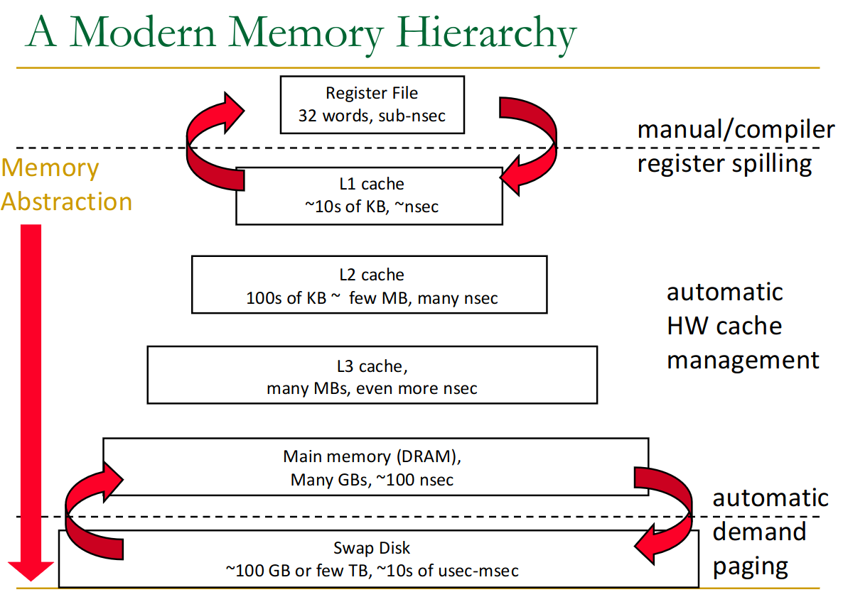
We want to keep the data that the processor needs as close to it as possible, in low-latency memory.

23.1 Locality

Programs tend to exhibit predictable access patterns (mainly composed of loops → regular).

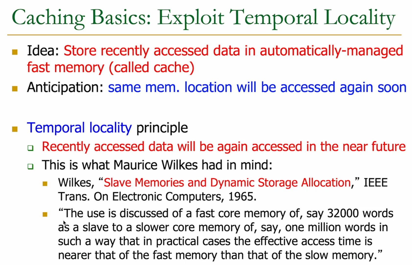
23.1.1 Temporal Locality

Temporal Locality: If a memory location is accessed, it is likely to be accessed again soon. This is common with loops and frequently used variables.

23.1.2 Spatial Locality

Spatial Locality: If a memory location is accessed, nearby memory locations are likely to be accessed soon. This is evident in sequential instruction execution and operations on contiguous data structures like arrays.

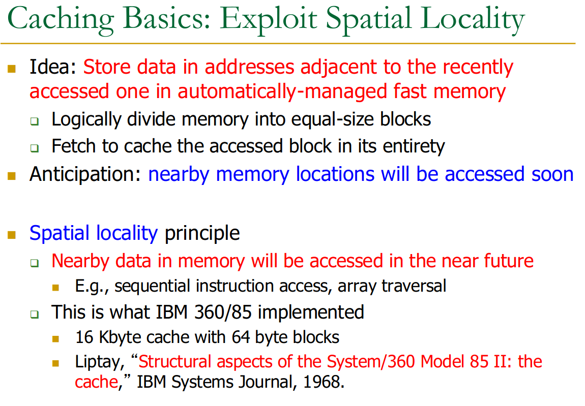
We load the entire block (and use the row-buffer) to exploit spatial locality.

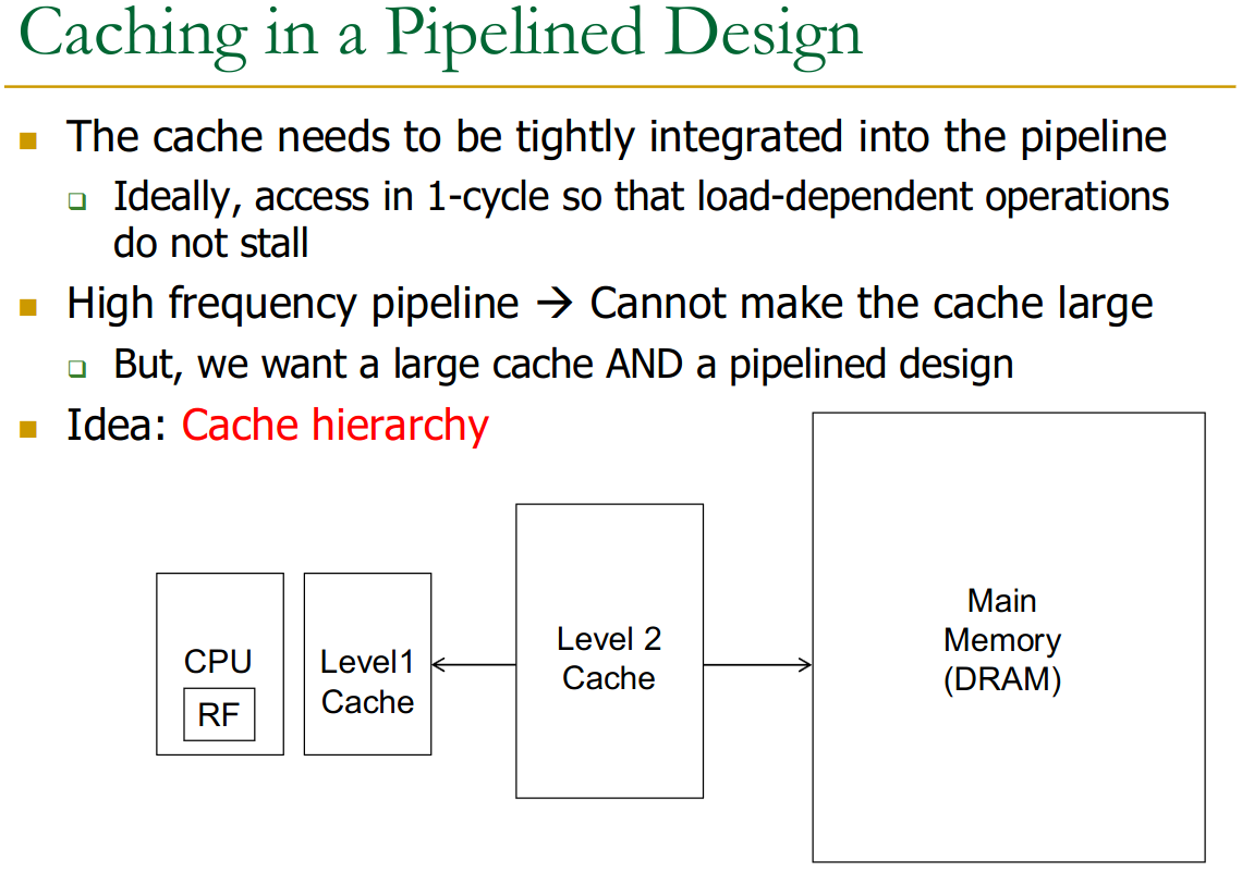
23.2 Hierarchy

Want fast access (with higher clock cycle of CPU) → smaller size of memory (otherwise latency increases) → we need the hierarchy.

Managing Memory in Cache:

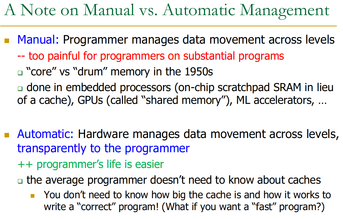
If you care about speed, you need to know (re-order data to optimise L1 hits, for ex). If only about correctness, no need.

23.3 Caching

23.3.1 Analysis of Caching

AMAT Deriving AMAT (Average memory access time) across a memory hierarchy.

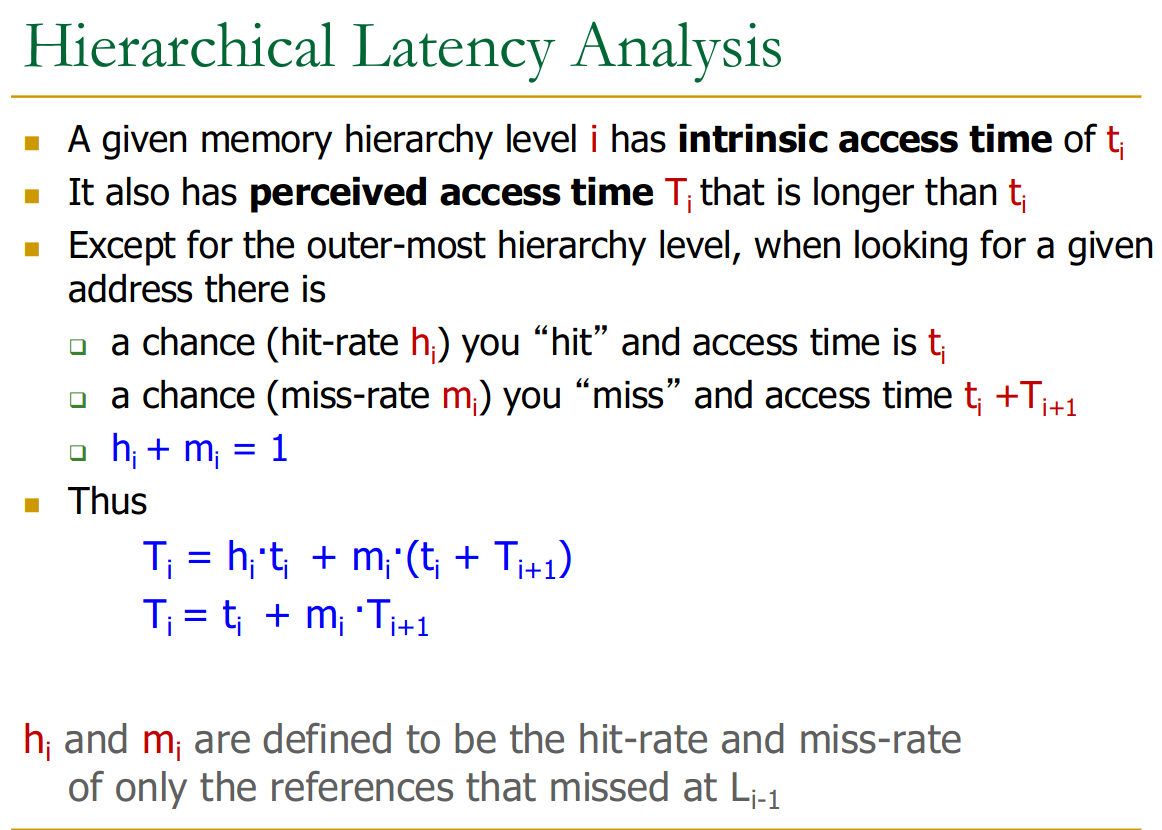
For a given level $i$:

• if we hit → takes $t_i$ intrinsic access time
• if we miss the cache, the time taken is $t_i+T_{i+1}$, ($t_i$ for checking the cache = realise there’s a miss + $T_{i+1}$ for actually getting the data from the next level)
  Notice this is a recursive definition. We don’t use $t_{i+1}$ since we aren’t sure to actually have a hit on the level $i+1$.

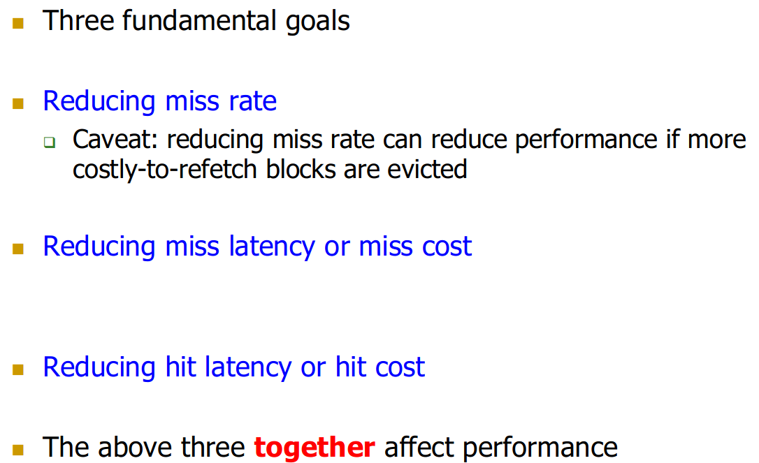
Goal We want to minimise this perceived latency for level $1$.

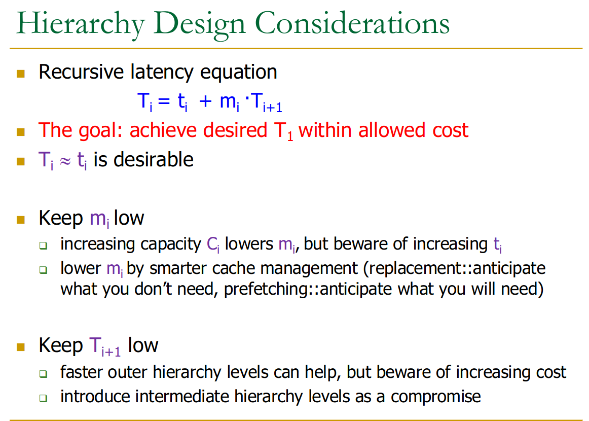
Either:

• Either we reduce missrate → increase capacity
  • but this also increases access latency
• keep outer hierarchy levels fast
  • more intermediate levels

Calculated Example

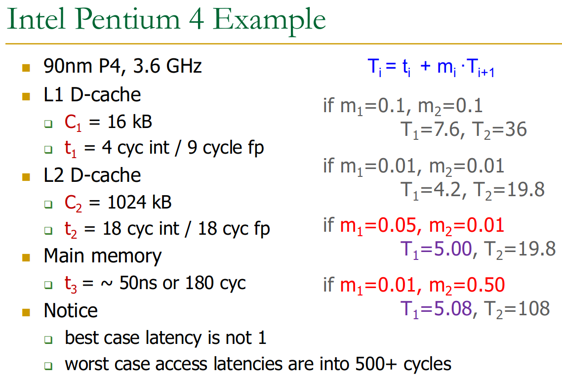
We just plug the numbers into the equation recursively, which gives:

$$T_1=t_1+m_1(t_2+m_2(t_3+0))=4+0.1(18+0.1(180))=7.6$$

We can try to decrease miss-rate on L1 by a lot and then have worse L2, L3, etc… and get same results as making all layers better.

23.3.2 Cache

Cache

Any structure that “memoizes” used or produced data to avoid repeating the long-latency operations to fetch from main memory.

Design we associate a tag with the cached data to indicate validity, address, etc…

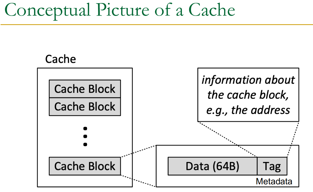
The tag store stores:

• valid bit (valid cache element)
• tag
• replacement policy bits (for LRU for ex)
• dirty (or modified) bit
  • for writes (write-through vs. write-back cache)

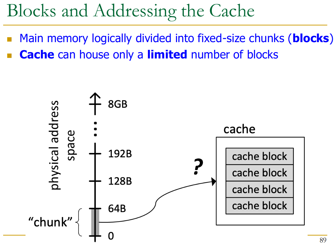
Cache Block (line)

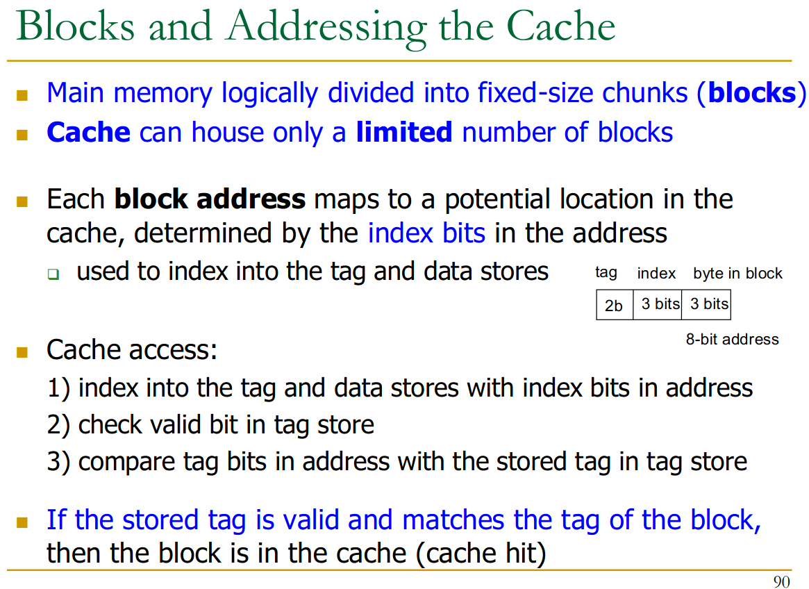
Unit of storage in the cache. Memory is logically divided into blocks that map to potential locations in the cache.

On a reference:

• HIT: if in cache, use cached data instead of accessing memory
• MISS: if not in cache → bring into cache
  • may have to evict other block

There are a few key design decisions to make:

• placement (see 23.4 Cache Addressing
• replacement (what data to remove)
• granularity (large or small blocks)
• write policy (what about writes)
• instructions / data → separate or not?

23.3.3 Metrics

We can measure the performance of our cache:

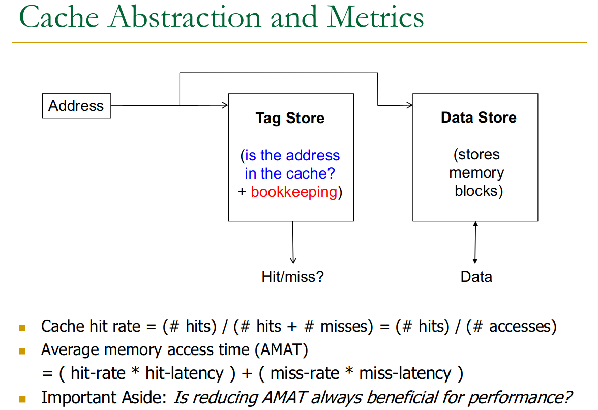
Improving Cache performance:

23.4 Cache Addressing

How do we map from main memory to our cache?

3 Options:

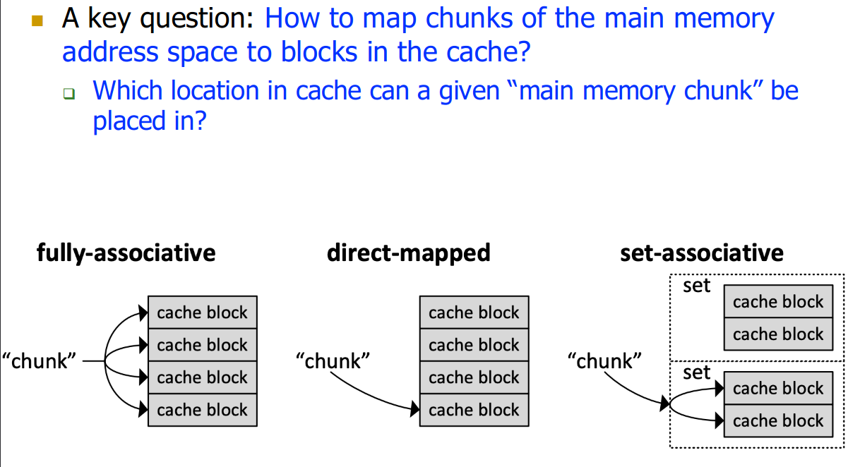
23.4.1 Direct Mapped

Direct Mapped Cache

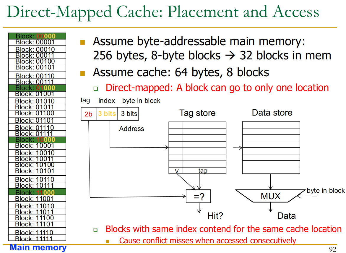
Direct-mapped cache basically uses address % cache-rows = row in cache to map from main memory into the cache.

Let $n=$ block-size and $m=$ # of blocks in cache.
This way, the memory is divided into “tag-groups” → groups of $m$ blocks that share the same tag (red bits).

• All blocks in a tag-group do not conflict in the memory

So the full address of a byte in memory is divided into:

• tag → ${\log }_2(\text{total mem size in bytes})-\text{index bits}-\text{byte in block bits}$
  • same as ${\log }_2(\text{main-mem size}/\text{\# blocks})$ bits
  • basically what is left over
• index → ${\log }_2(m)$ bits so for 8 blocks = 3 bits
  • this addresses the rows inside the cache
• byte in block → ${\log }_2(n)$ so for 8 byte blocks = 3 bits
  • this chooses the right byte from the cache-row

This (modulo over addresses, like rotating) is a sensible way to design the cache because it exploits temporal locality

• addresses close together map to different cache-rows
• we only need to compare the tag of one row → very fast

But what if the stride of our array data = # of blocks → 0% hit rate.

23.4.2 Set-Associative

Instead of each index having only 1 cache-row, we have multiple rows associated with them. Thus even when two entries with different tag bits come in (such as in a strided array), we can cache both.

Example Calculation

• Continuing the 64-byte cache, 8-byte block example:
  • If it’s 2-way set-associative, the number of sets S=Total Cache Blocks/N=8/2=4 sets.
  • Index bits needed $\log 2(S)=\log 2(4)=2$ bits.
  • Tag bits = Total - Index - Offset = $8-2-3=3$ bits.
• Now, two memory blocks that map to the same set (e.g., set 0) can co-exist in the cache, one in Way 0 and one in Way 1 of that set.

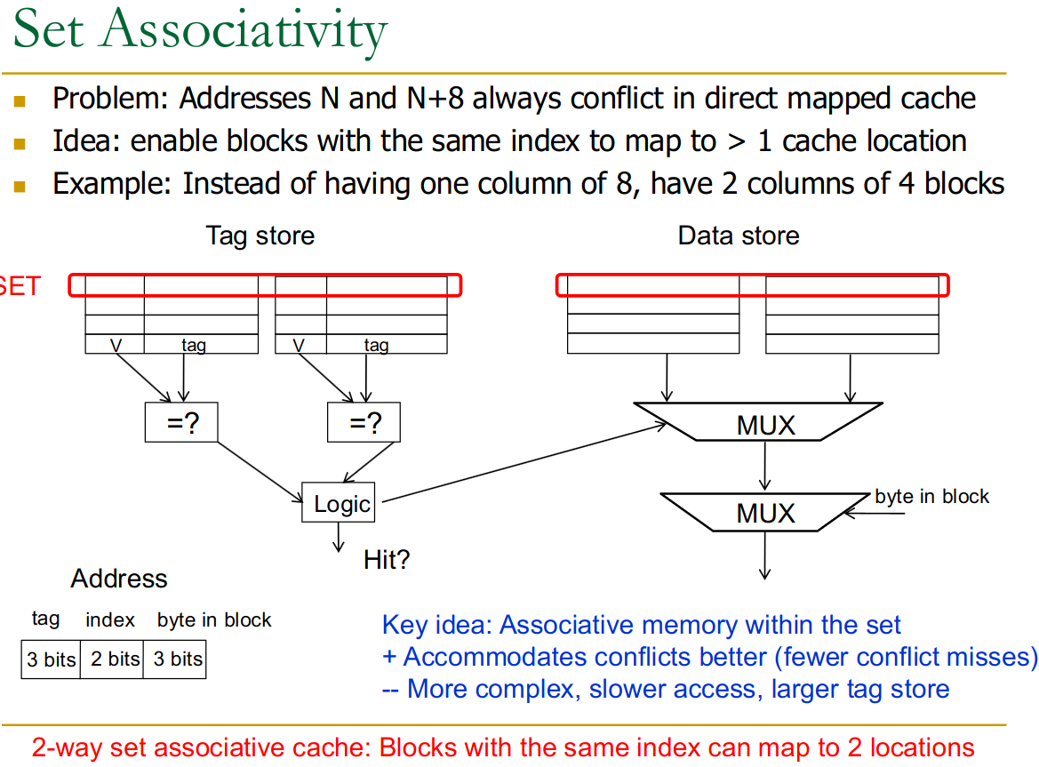
The issues is that now we need to compare as many tags as we have elements in each set → higher cost.

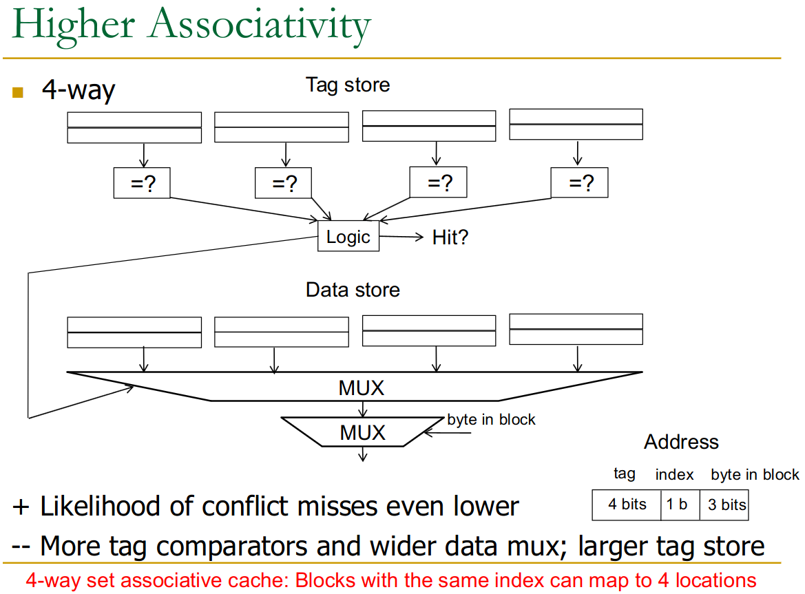
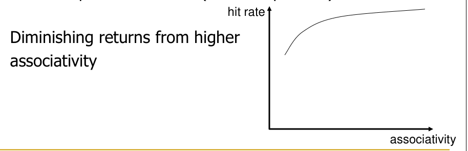
Higher associativity:

• higher hit rate
• slower access time (more comparisons)
• more expensive hardware

There are also diminishing returns.

23.4.3 Fully Associative

For a fully associative cache, we need to compare all tag bits. Thus we don’t need any index bit anymore.

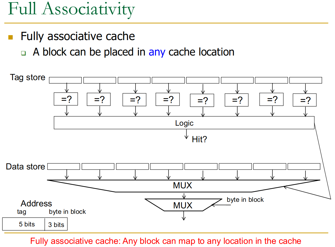
→ Eliminates conflict misses entirely. Misses are only compulsory or capacity.

But most expensive and potentially slowest due to the large number of comparators.

23.5 Management in Set-Associative Cache

When a block can go into multiple ‘ways’ within a set, policies are needed to manage these ways. These policies revolve around three key decisions:

1. Insertion: When a new block is brought into a set (cache fill), where is it placed (e.g., in the Most Recently Used - MRU - position)? Should it even be inserted if it’s predicted to have no reuse?
2. Promotion: If a block already in the set is accessed (a hit), how is its priority updated (e.g., promoted to MRU)?
3. Eviction/Replacement: If a set is full and a new block needs to be brought in (a miss), which existing block should be removed?

23.5.1 Eviction / Replacement Policies

The theoretically optimal replacement policy (also called Belady’s OPT or MIN) is to evict the block that will be referenced furthest in the future = guarantees minimum miss-rate
→ not practically implementable.
Note: it’s not optimal for execution time (passing over cache might be faster if data not used again)

There are a number of eviction policies:

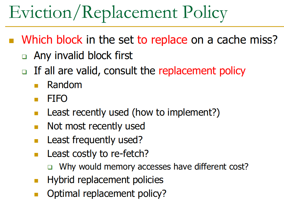
The goal of most policies would be Reducing miss-rate. But that is not actually always optimal → some misses more costly than others (due to stall time in CPU, depending on OoO).

23.5.2 LRU

LRU: LRU is commonly used, as it exploits the loop structure of most programs.

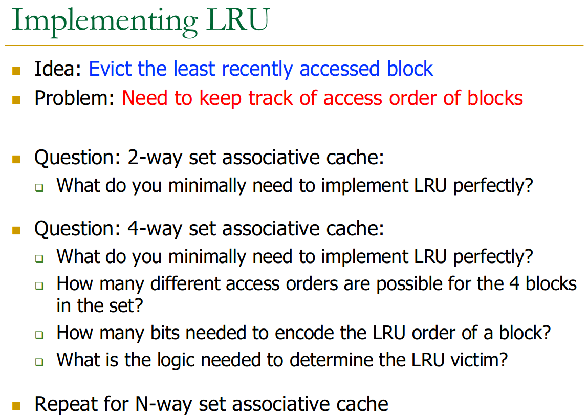
→ but LRU expensive to implement for highly associative caches

• for associativity $N$ requires encoding $N!$ possible orders → high bit requirements.

That is why we use LRU approximations:

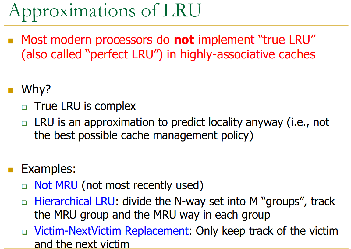
LRU is already an approximation → so no need to even implement LRU perfectly.

Edge-cases: Comparing LRU vs Random

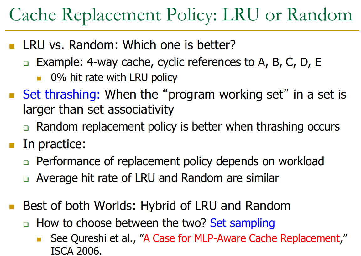
When set-thrashing occurs, random performs better since we might evict exactly the blocks we need next
→ throws away the beginning of the loop (A-B-C-D-E, looping around)
so we have to re-fetch on every loop

23.6 Cache Write Policies

23.6.1 Write-Through vs. Write-Back

When do you write to main memory:

• Write-through = when modified
• write-back = when evicted

This determines when modified data is propagated to the next lower memory level.

• Write-Through: Data is written to the current cache level and simultaneously to the next lower level.

  • Pros: Simpler design, main memory is always up-to-date
    → simplifies coherence
  • Cons: High bandwidth usage, no write combining
    • multiple writes to the same block go to memory individually
      → write locality!

• Write-Back: Data is written only to the current cache level, and the block is marked “dirty.” The modified block is written to the next level only when it’s evicted.

  • Pros: Allows write combining, reducing bandwidth and energy by consolidating multiple writes to a block into a single write-back upon eviction.
  • Cons: More complex (needs dirty bits), next level isn’t always up-to-date (complicates coherence).

Most high-performance caches today use write-back.

23.6.2 Write-Allocate vs. No-Write-Allocate

Do we allocate on Write-Miss → i.e. on a store instruction.

This policy applies on a write miss.

• Write-Allocate (Fetch-on-Write): On a write miss, the block is first fetched into the cache, and then the write is performed.
  • Pros: Allows subsequent writes to the block to be combined (if write-back is used).
  • Cons: Fetches the entire block even if only a small part is written, potentially inefficient.
• No-Write-Allocate (Write-Around): On a write miss, the block is not brought into the cache. The write goes directly to the next lower level.
  • Pros: Conserves cache space if the locality of written blocks is low.

The common combination is write-back with write-allocate.

23.6.3 Subblocked (Sectored) Caches

To handle writes more efficiently, especially when write granularity (e.g., 4 bytes) is much smaller than block granularity (e.g., 64 bytes):

• Idea: Divide a cache block into smaller subblocks or sectors. The block has one tag, but each subblock has its own valid and dirty bits.
• Benefits:
  • Allows writing to a subblock without fetching the entire block (if it’s a full subblock write).
  • Reduces data transfer on misses if only specific subblocks are needed.
  • Finer granularity for cache management.
• Drawbacks: More complex design due to additional valid/dirty bits.

23.7 Instruction Cache

Do we store instructions and data into separate caches, or do we combine them?

Depends on the hierarchy:

• First-Level (L1) Caches: Almost always split into separate Instruction (I-cache) and Data (D-cache).
  • Reason: Primarily due to pipeline design. Instructions are fetched in early pipeline stages, and data is accessed in later stages. Separate caches allow these accesses to occur in parallel without structural hazards.
• Outer-Level (L2, L3) Caches: Usually unified, storing both instructions and data.
  • Benefit: Better overall cache utilization through dynamic sharing of space.

23.8 Multi-Level Cache Management

Cache design and management varies by the level → trade-offs are difference in the levels:

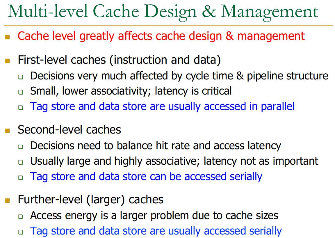
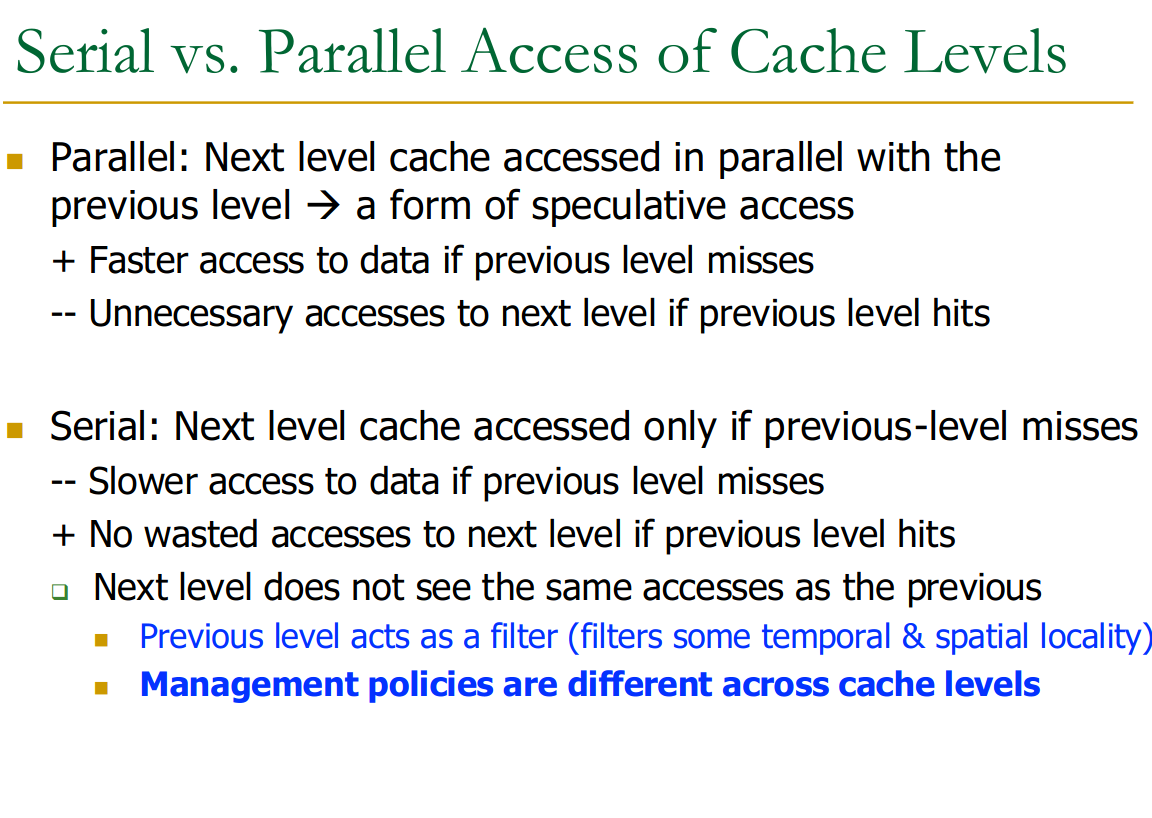
23.8.1 Parallel vs. Serial Accesses

We can reduce latency of fetching by accessing higher levels in parallels:

23.8.2 Decisions

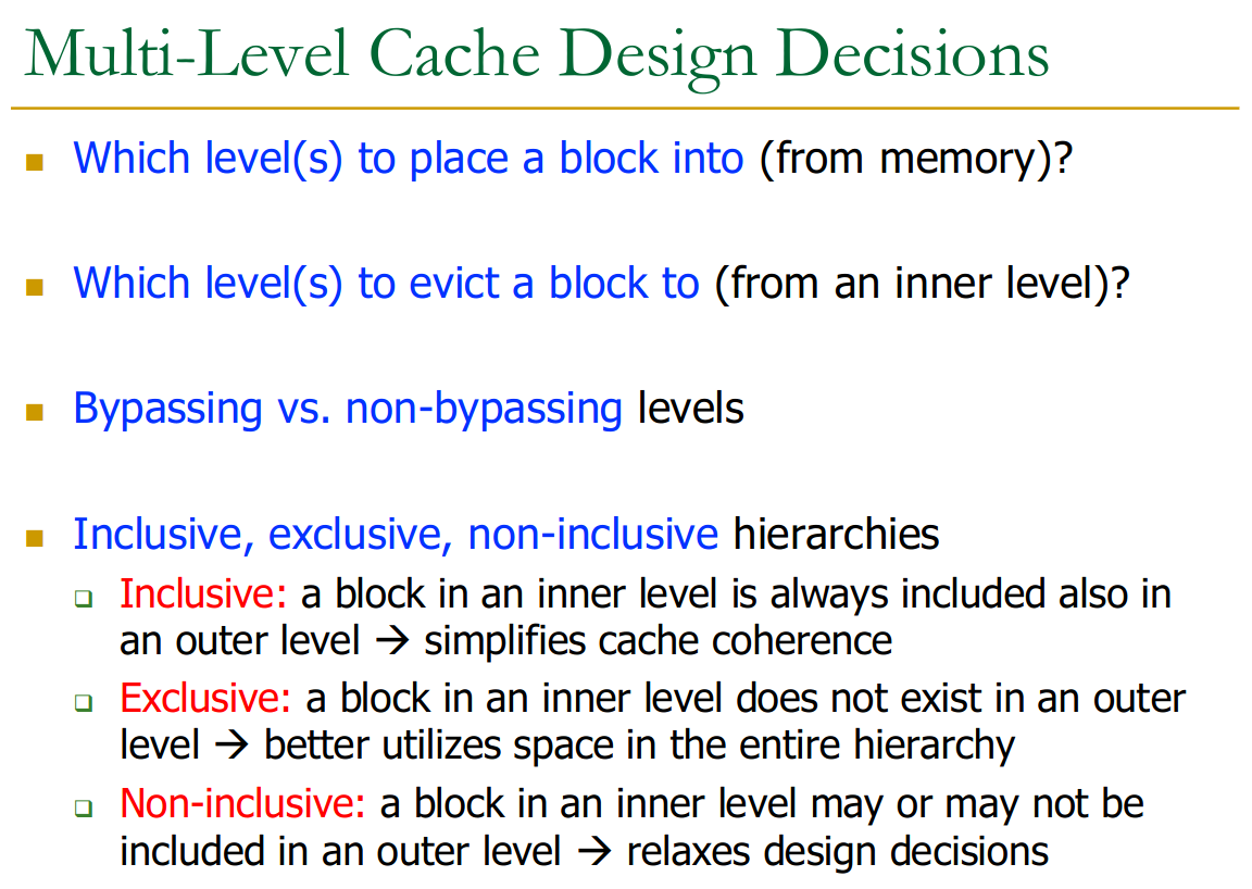
bypassing is interesting → makes Belady’s OPT non-optimal under those assumptions.

23.9 Cache Performance

The performance depends on:

• Cache size

• block size

• associativity

• replacement policy

• insertion policy

• promotion policy

23.9.1 Cache Size

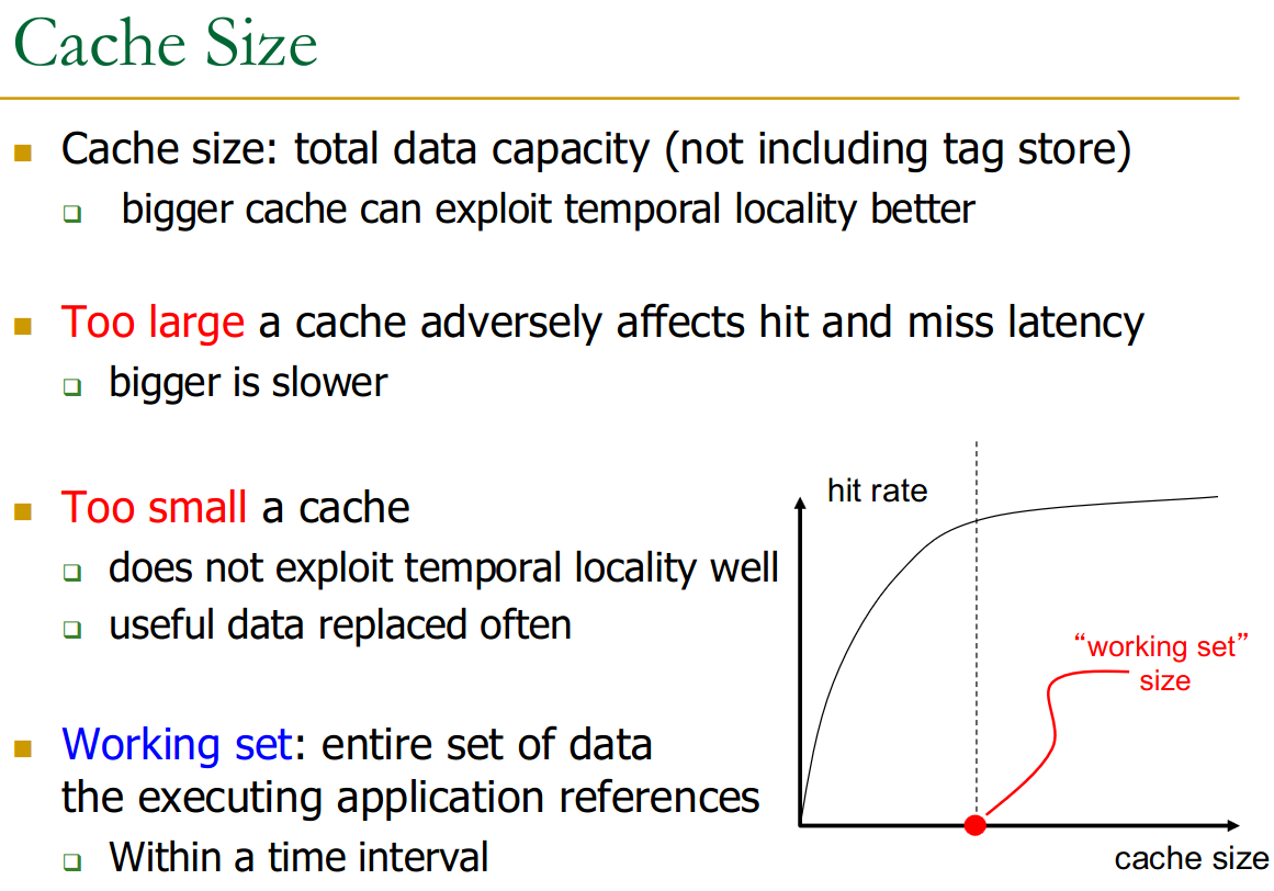
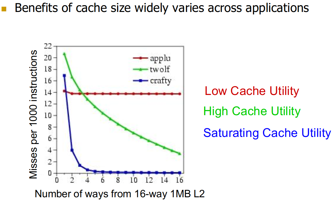
This varies very wildly with access patterns in applications.

23.9.2 Block Size

There are also trade-offs associated with block-size:

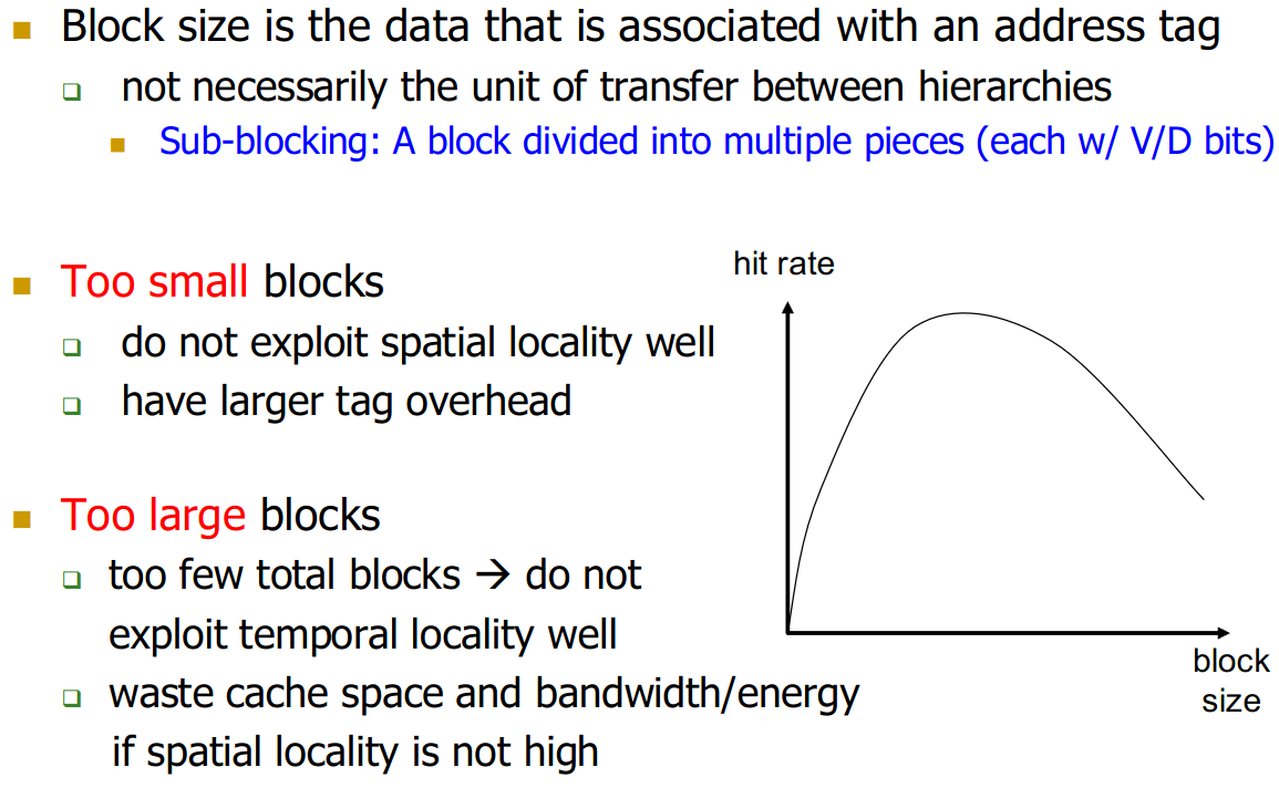
→ block size did not increase substantially, unlike cache size. Smaller = more flexible for software.

Subblocking:

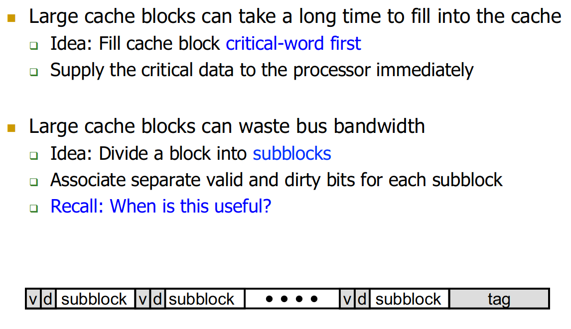
Don’t load block all at once → load them out of order:

• Critical word = word requested by program.

23.9.3 Associativity

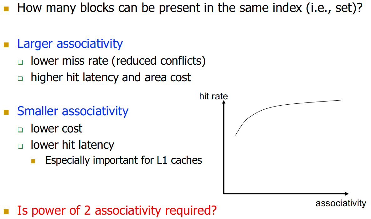
power of 2 associativity not required → no bit indexing into the set, $N$ only determines the number of mux / comparators you need
→ intel actually has 12-way

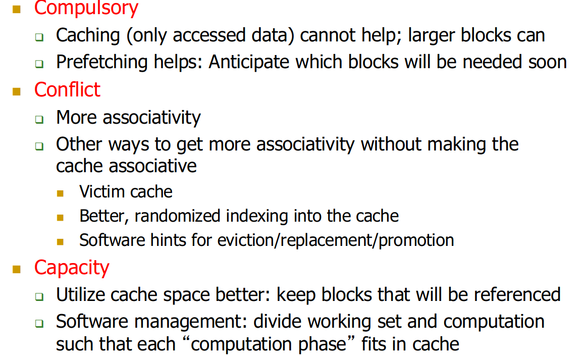
23.10 Classifying Cache Misses

1. Compulsory (Cold): First-time access to a block.

   1. cannot be eliminated
      1. maybe pre-fetching…

2. Capacity: Cache is too small for the working set, even if fully associative.

3. Conflict: Misses due to too many blocks mapping to the same set in direct-mapped or set-associative caches, even if overall capacity is sufficient.

How to reduce them:

23.11 Software Approach for Higher Hit Rate

23.11.1 Restructure Data Accesses

Loop Interchanging Row-major / column-major → loop interchanging.

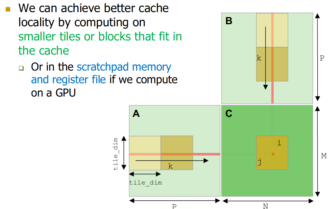
Blocking (Tiling) Divide large data-structures (like matrices) into smaller blocks that fit into cache

• computation then tile by tile

Otherwise, if $P$ too large, we basically always miss after some amount of rows…

23.11.2 Restructuring Data Layout

We can store data in a smarter way to allow caching more of the important data fields in a list of objects.

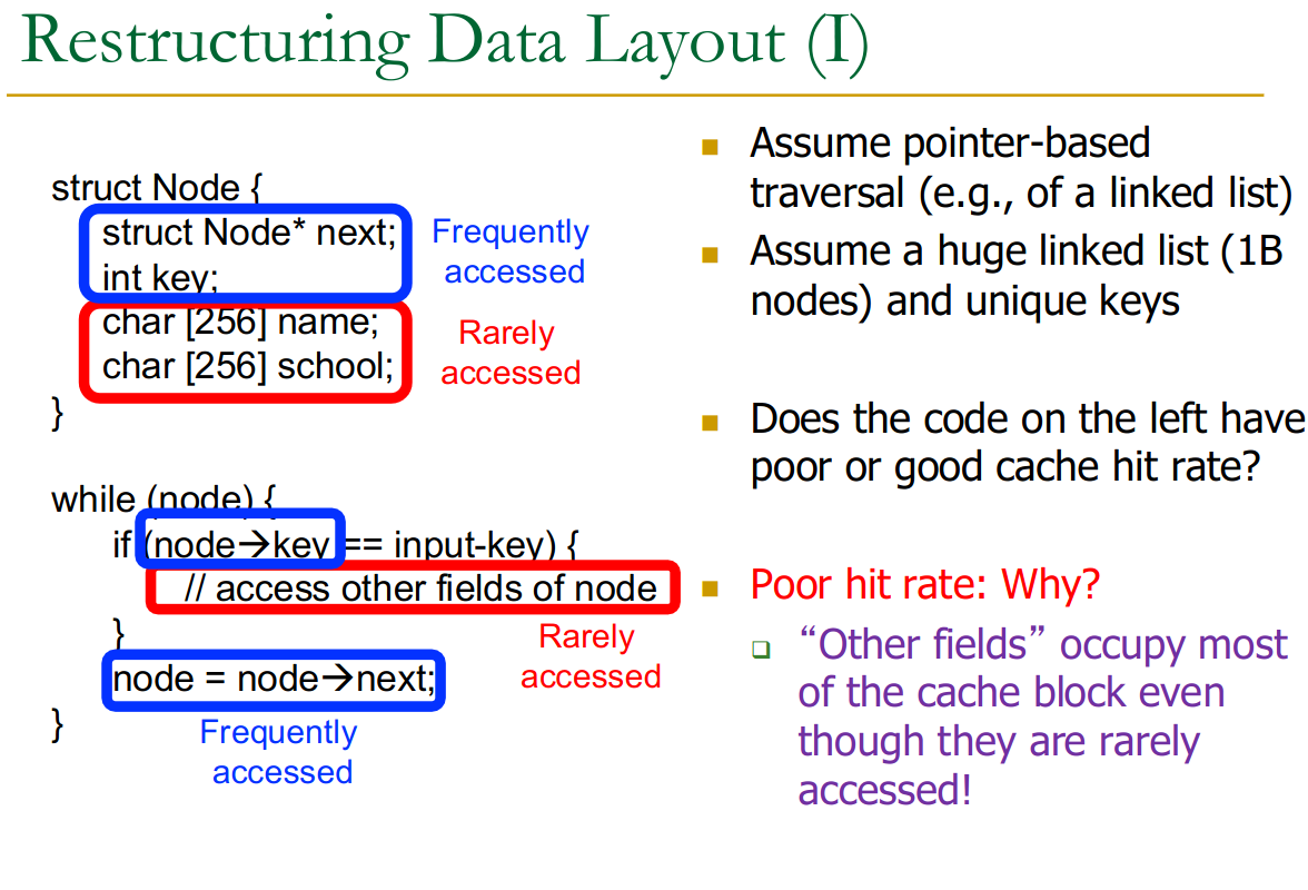
Separate into extra table → hot data vs. cold data

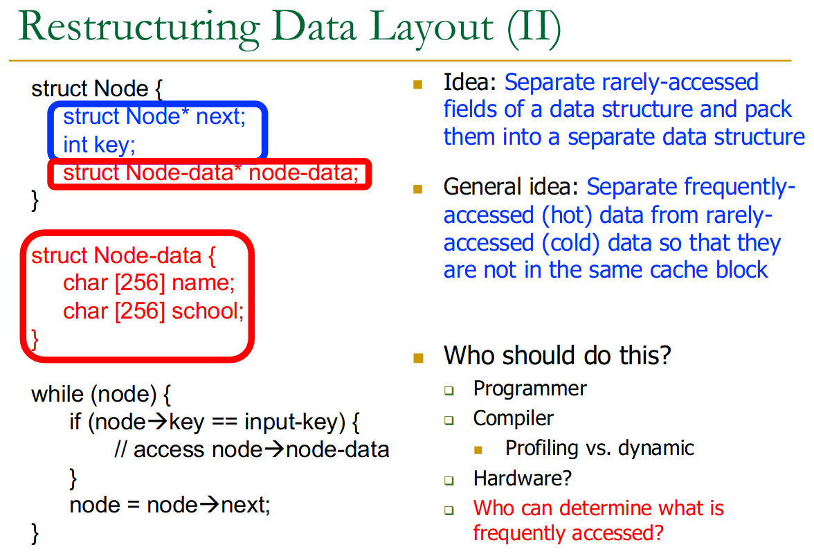
Who should do this? Programmer / Compiler / Hardware?